%%html
<style>
.emph4780 {
    font-weight: bold;
    color: navy;
}
.red4780 {
    font-weight: bold;
    color: red;
}
.diagram4780 {
    display: block;
    margin-left: auto;
    margin-right: auto;
}
.diagram4780 img {
    width: 80%;
    padding: 16px;
}
#myimg1 {
    display: inline;
    margin-top: 0px;
}
#myimg2 {
    display: inline;
    margin-top: 0px;
}
</style>

Low-Dimensional Structure to the Rescue

If the data lies in a low-dimensional submanifold, then we

import numpy as np
import sys
import matplotlib
import matplotlib.pyplot as plt
from scipy.io import loadmat
import time
from pylab import *
from helperfunctions import knn_demo_1, knn_demo_2, knn_demo_3, curse_demo_1, curse_demo_2, curse_demo_3
from matplotlib.animation import FuncAnimation

%matplotlib notebook

Lecture 3: k-Nearest Neighbors

CS4780 — Introduction to Machine Learning

$\newcommand{\R}{\mathbb{R}}$ $\newcommand{\norm}[1]{\left\|#1\right\|}$

The k-Nearest Neighbors Algorithm

• Assumption: Nearby inputs have similar outputs.

• Hypothesis: Given a test input $x$, output the most common label among its $k$ most-similar training inputs.

  • 1-nearest neighbors is simpler: just output the label of the most-similar training input.

k-Nearest Neighbors Illustration

k-NN Formally

• Start with training set $(x_1, y_1), \ldots, (x_n, y_n)$
• Given input $x_{\text{test}}$
• Compute $d_i = \operatorname{dist}(x_{\text{test}}, x_i)$ for all $i \in \{1, \ldots, n\}$
• Compute $S$, where $S \subset \{1,\ldots, n\}$, $|S| = k$, and $$i \in S, \; j \notin S \; \rightarrow \; d_i \le d_j$$
• Output the most common label $$h(x_{\text{test}}) = \arg \max_{y \in \mathcal{Y}} \; \left|\left\{ i \in S \middle| y_i = y \right\} \right|$$

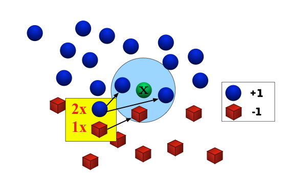
What should we do in case of a tie?

• Choose at random/arbitrarily
• Fall back to $k - 1$; go up to $k+1$

k-NN For Regression

• Start with training set $(x_1, y_1), \ldots, (x_n, y_n)$
• Given input $x_{\text{test}}$
• Compute $d_i = \operatorname{dist}(x_{\text{test}}, x_i)$ for all $i \in \{1, \ldots, n\}$
• Compute $S$, where $S \subset \{1,\ldots, n\}$, $|S| = k$, and $$i \in S, \; j \notin S \; \rightarrow \; d_i \le d_j$$
• Output the average of the labels $$h(x_{\text{test}}) = \frac{1}{k} \sum_{i \in S} y_i.$$

What distance function should we use?

Most common distance: the Euclidean distance $$\operatorname{dist}(u,v) = \| u - v \|_2 = \sqrt{ \sum_{i=1}^d (u_i - v_i)^2 }$$

Also popular: the taxicab norm (a.k.a. Manhattan norm) $$\operatorname{dist}(u,v) = \| u - v \|_1 = \sum_{i=1}^d |u_i - v_i|$$

The Minkowski distance (a.k.a. $\ell_p$ space)

For parameter $p \ge 1$

$$\operatorname{dist}(u,v) = \| u - v \|_p = \left( \sum_{i=1}^d |u_i - v_i|^p \right)^{1/p}$$

Generalizes many other norms, including the popular $\ell_2$ (Euclidean), $\ell_1$ (taxicab), and $\ell_{\infty}$ (max norm).

• Many other norms are used in practice, including learned norms.
• Which norm to use will depend on your task.

%matplotlib notebook
knn_demo_1()

%matplotlib notebook
knn_demo_2()

Click on the images above, to cycle through the test images.

knn_demo_3()

interactive(children=(IntSlider(value=1, description='k', max=19, min=1, step=2), Output()), _dom_classes=('wi…

Bayes Optimal Classifier

The Bayes Optimal Classifier is the hypothesis

$$h_{\operatorname{opt}}(x) = \arg \max_{y \in \mathcal{Y}} \; \mathcal{P}(y | x) = \arg \max_{y \in \mathcal{Y}} \; \mathcal{P}(x, y).$$

• It picks the label that is most likely in the source distribution $\mathcal{P}$.
• This is the "best" hypothesis possible for the task, and its loss/error measures the best you could do.

Bayes Optimal Classifier: A Silly Example

• Suppose you are playing your favorite RPG and you get attacked by a wolf-like creature.
• You want to predict whether the creature is a wolf or a werewolf.
  • Wolves occur with probability $50%$, and werewolves $50%$.
• You observe the amount of damage the creature did, and you know how much damage wolves and werewolves do.
  • A wolf deals damage equal to a roll on a six-sided dice plus one.
  • A werewolf deals damage equal to the sum of the rolls on two four-sided dice.

Bayes Optimal Classifier: Conditional Probability

Conditional probability of damage $x$ conditioned on label $y$.

Damage	Wolf (1d6+1)	Werewolf (2d4)
2	1/6	1/16
3	1/6	1/8
4	1/6	3/16
5	1/6	1/4
6	1/6	3/16
7	1/6	1/8
8	0	1/16

Bayes Optimal Classifier: Joint Probability

Joint density: $\mathcal{P}(x,y) = \mathcal{P}(x | y) \mathcal{P}(y) = \mathcal{P}(x | y) \cdot \frac{1}{2}$

Damage	Wolf (1d6+1)	Werewolf (2d4)
2	1/12	1/32
3	1/12	1/16
4	1/12	3/32
5	1/12	1/8
6	1/12	3/32
7	1/12	1/16
8	0	1/32

Bayes Optimal Classifier: The Hypothesis

Always guess the label with the highest probability.

Damage	Wolf (1d6+1)	Werewolf (2d4)	Bayes Optimal Classifier Prediction
2	1/12	1/32	Wolf
3	1/12	1/16	Wolf
4	1/12	3/32	Werewolf
5	1/12	1/8	Werewolf
6	1/12	3/32	Werewolf
7	1/12	1/16	Wolf
8	0	1/32	Werewolf

Does this being "optimal" mean we get it right all the time?

Bayes Optimal Classifier: What's the Error Rate?

We get it wrong when the true label disagrees with our prediction.

Damage	Wolf (1d6+1)	Werewolf (2d4)	Bayes Optimal Classifier Prediction
2	1/12	1/32	Wolf
3	1/12	1/16	Wolf
4	1/12	3/32	Werewolf
5	1/12	1/8	Werewolf
6	1/12	3/32	Werewolf
7	1/12	1/16	Wolf
8	0	1/32	Werewolf

$\operatorname{error} = \frac{1}{32} + \frac{1}{16} + \frac{1}{12} + \frac{1}{12} + \frac{1}{12} + \frac{1}{16} + 0 = \frac{13}{32} \approx 41\%.$

Bayes Optimal Classifier: Take-Away

• We care about the Bayes Optimal Classifier because it gives us a "best-case" baseline against which we can compare our hypothesis' performance.
  • Although only in theory: in practice we don't know $\mathcal{P}$
  • Expected Error of Bayes Optimal Classifier is lowest possible.
  • Is the loss of the Bayes Optimal Classifier always the lowest possible?

Best Constant Predictor

Another important baseline is the Best Constant Predictor.

$$h(x) = \arg \max_{y \in \mathcal{Y}} \; \mathcal{P}(y).$$

• Just guesses the label that occurs the most often.
• This predicts completely independently of $x$.
• Important for debugging: You should always be able to show that your classifier performs significantly better on the test set than the Best Constant Predictor.

How does k-NN compare to the Bayes Optimal Classifier?

We can bound the error of 1-NN relative to the Bayes Optimal Classifier.

• Here we'll follow the original proof in Cover and Hart (1967).

Lemma: Convergence of the Nearest Neighbor

Suppose that $(\mathcal{X}, \operatorname{dist})$ is a separable metric space.

• A metric space is separable if there is countable subset of $\mathcal{X}$ that is dense in the space, i.e. a sequence that comes arbitrarily close to every point in the space.
• In particular, $\mathbb{R}^d$ is separable.

Let $x_{\text{test}}$ and $x_1, x_2, \ldots$ be independent identically distributed random variables over $\mathcal{X}$. Then almost surely (i.e. with probability $1$)

$$\lim_{n \rightarrow \infty} \; \arg \min_{x \in \{x_1, \ldots, x_n\}} \operatorname{dist}(x, x_{\text{test}}) = x_{\text{test}}.$$

Proof Outline: Case 1

Consider the case where any ball of radius $r$ centered around $x_{\text{test}}$ has positive probability.

Then, no matter now close the current nearest neighbor is to $x_{\text{test}}$, every time we draw a fresh sample $x_i$ from the source distribution, with some probability it will be closer than the nearest neighbor currently in the distribution.

This implies that the distance diminishes to $0$ with probability $1$.

Proof Outline: Case 2

Consider the case where there is some ball of radius $r$ centered around $x_{\text{test}}$ that has probability zero in the source distribution.

But this must happen with zero probability in the random selection of $x_{\text{test}}$.

• Why? Let $Z$ be the set of all points in $\mathcal{X}$ that have the property that they are the center of some ball with zero probability. Then because $\mathcal{X}$ is separable, we can cover $Z$ with the union of a countable number of balls with zero probability. So $Z$ itself must have zero probability.

• You defintely don't need to know this topology stuff for CS4/5780, but I think it's good to mention it so you have some intuition about when NN might fail on exotic spaces.

Bounding the Error of 1-NN

Let $x_{\text{test}}$ denote a test point randomly drawn from $\mathcal{P}$. Let $\hat x_n$ (also a random variable) denote the nearest neighbor to $x_{\text{test}}$ in an independent training dataset of size $n$.

The expected error of the 1-NN classifier is $$ \operatorname{error}_{\text{1-NN}} = \mathbf{E}\left[ \sum_{y \in \mathcal{Y}} \mathcal{P}(y | \hat x_n) \left(1 - \mathcal{P}(y | x_{\text{test}})\right) \right]. $$ This is the sum over all labels $y$ of the probability that the prediction will be $y$ but the true label will not be $y$.

Bounding the Error of 1-NN in the limit

Taking the limit as $n$ approaches infinity, the expected error is \begin{align*} \lim_{n \rightarrow \infty} \; \operatorname{error}_{\text{1-NN}} &= \lim_{n \rightarrow \infty} \; \mathbf{E}\left[ \sum_{y \in \mathcal{Y}} \mathcal{P}(y | \hat x_n) \left(1 - \mathcal{P}(y | x_{\text{test}})\right) \right] \\&= \mathbf{E}\left[ \sum_{y \in \mathcal{Y}} \mathcal{P}(y | x_{\text{test}})) \left(1 - \mathcal{P}(y | x_{\text{test}})\right) \right] \end{align*}

Comparing to the Bayes Optimal Classifier

Let $\hat y$ denote the prediction of the Bayes Optimal Classifier on $x_{\text{test}}$. \begin{align*} \lim{n \rightarrow \infty} \; \operatorname{error}{\text{1-NN}} &= \mathbf{E}\left[ \mathcal{P}(\hat y | x{\text{test}}) \left(1 - \mathcal{P}(\hat y | x{\text{test}})\right) \right] \&\hspace{2em}+ \mathbf{E}\left[ \sum{y \ne \hat y} \mathcal{P}(y | x{\text{test}})) \left(1 - \mathcal{P}(y | x{\text{test}})\right) \right] \&\le \mathbf{E}\left[ 1 \cdot \left( 1 - \mathcal{P}(\hat y | x{\text{test}}) \right) \right] + \mathbf{E}\left[ \sum{y \ne \hat y} 1 \cdot \mathcal{P}(y | x{\text{test}})) \right] \&=

2 \mathbf{E}\left[ 1 - \mathcal{P}(\hat y | x_{\text{test}})\right]
=
2 \operatorname{error}_{\text{Bayes}}. 

\end{align*}

Conclusion: 1-NN is no more than a factor-of-2 worse

$$\lim_{n \rightarrow \infty} \; \operatorname{error}_{\text{1-NN}} \le 2 \operatorname{error}_{\text{Bayes}}.$$

...in the limit...and results in-the-limit can be suspicious because they don't tell us how fast we converge

k-NN is limited by The Curse of Dimensionality!

k-NN works by reasoning about how close together points are.

In high dimensional space, points drawn from a distribution tend not to be close together.

• Need to draw a very large number of points before you'll get two that are particularly close to each other.

First, let's look at some random points and a line in the unit square.

fig = plt.figure(); X=np.random.rand(50,2);
plot(X[:,0],X[:,1],'b.'); plot([0,1],[0.5,0.5],'r-');  axis('square'); axis((0,1,0,1));

Consider what happens when we move to three dimensions. The points move further away from each other but stay equally close to the red hyperplane.

(fig,animate) = curse_demo_1()
ani = FuncAnimation(fig, animate,arange(1,100,1),interval=10);

curse_demo_2()

curse_demo_3()

Curse of Dimensionality

• The pairwise distance between two points in a unit cube (or sphere, or from a unit Gaussian) increases with dimension.

  • Classifiers that use pairwise distances can have no points nearby a given test point.
  • Which point is the nearest can depend on measurement noise.

• In comparison, the distance to a hyperplane does not increase.

Low-Dimensional Structure to the Rescue

If the data lies in a low-dimensional submanifold, then we can still use low-dimensional methods even in higher dimensions.

• E.g. human faces

Reminders

• Please finish the prelim exam (placement quiz)!

• First homework is out tonight!

  • Work in groups of up to two (2)!