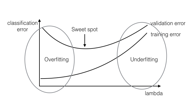
Figure 1: overfitting and underfitting
Underfitting: The classifier learned on the training set is not expressive enough (i.e. too simple) to even account for the data provided. In this case, both the training error and the test error will be high, as the classifier does not account for relevant information present in the training set.
Overfitting: The classifier learned on the training set is too specific, and cannot be used to accurately infer anything about unseen data. Although training error continues to decrease over time, test error will begin to increase again as the classifier begins to make decisions based on patterns which exist only in the training set and not in the broader distribution.
Figure 1: overfitting and underfitting
Divide data into training and validation portions. Train your algorithm on the "training" split and evaluate it on the "validation" split, for various value of $\lambda$ (Typical values: 10-5 10-4 10-3 10-2 10-1 100 101 102 ...).
k-fold cross validationDivide your training data into $k$ partitions. Train on $k-1$ of them and leave one out as validation set. Do this $k$ times (i.e. leave out every partition exactly once) and average the validation error across runs. This gives you a good estimate of the validation error (even with standard deviation). In the extreme case, you can have $k=n$, i.e. you only leave a single data point out (this is often referred to as LOOCV- Leave One Out Cross Validation). LOOCV is important if your data set is small and cannot afford to leave out many data points for evaluation .
Telescopic searchDo two searches: 1st, find the best order of magnitude for $\lambda$; 2nd, do a more fine-grained search around the best $\lambda$ found so far. For example, first you try $\lambda=0.01,0.1,1,10,100$. It turns out 10 is the best performing value. Then you try out $\lambda=5,10,15,20,25,...,95$ to test values "around" $10$.
Grid and Random searchIf you have multiple parameters (e.g. $\lambda$ and also the kernel width $\sigma$ in case you are using a kernel) a simple way to find the best value of both of them is to fix a set of values for each hyper-parameter and try out every combination. One downside of this method is that the number of settings you need to try out grows exponentially with the number of hyper-parameters. Also, if your model is insensitive to one of the parameters, you waste a lot of computation by trying out many different settings for it. An variant of grid-search is random search. Instead of selecting hyper-parameters on a pre-defined grid, we select them randomly within pre-defined intervals (See Figure 2). One advantage is that if for example the algorithm is somewhat insensitive to exact values of $\lambda$ and sensitive to $\sigma$, then by performing e.g. $6\times 6$ grid search you will learn little from varying $\lambda$ six times and you only explore six values of $\sigma$. However, if you do random search, again the changes in $\lambda$ may not matter too much, but now you are exploring 36 (!) different values of $\sigma$.
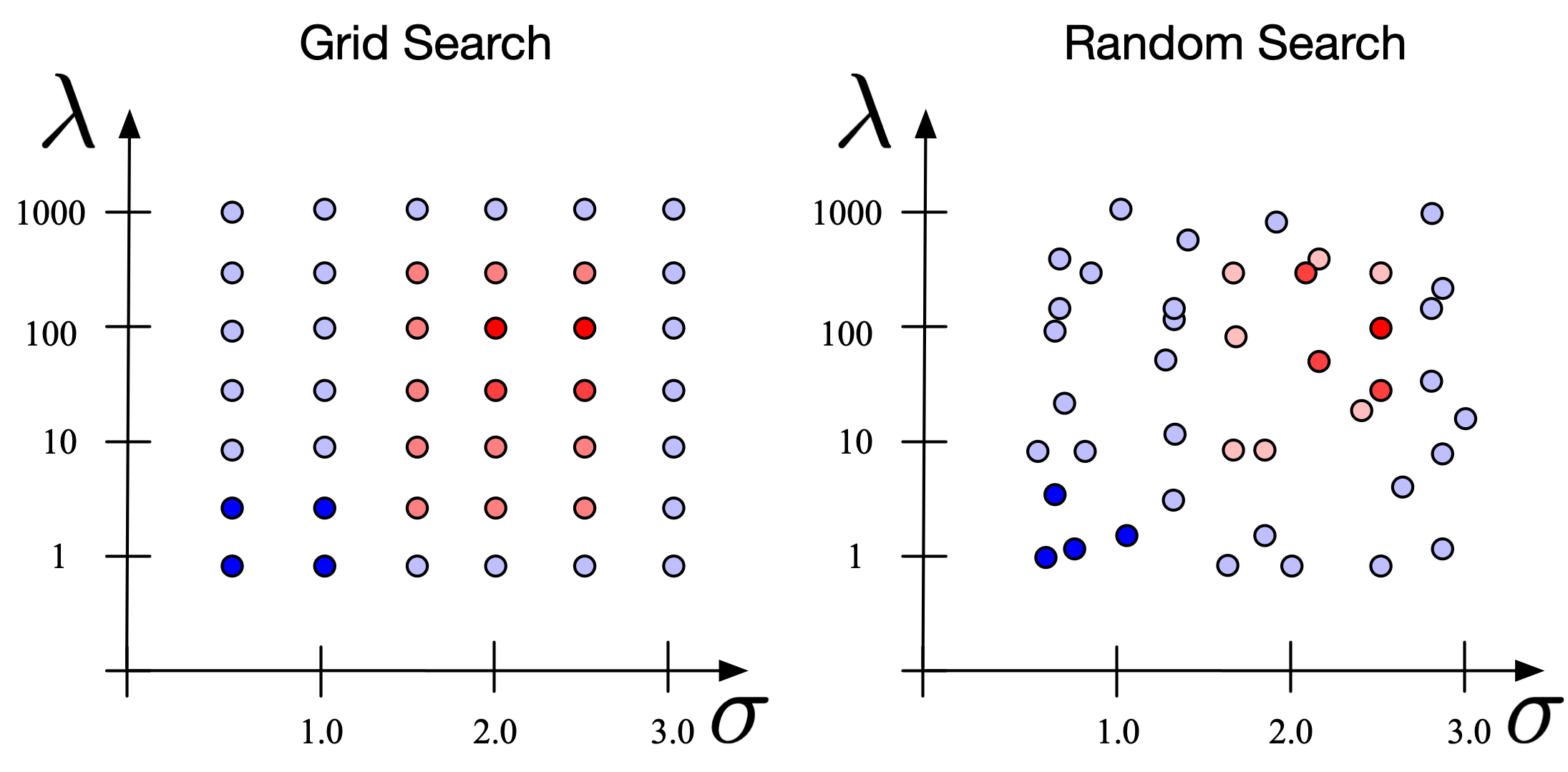
Figure 2: Grid Search vs Random search (red indicates lower loss, blue indicates high loss). One advantage of Random Search is that significantly more values of each individual hyper-parameter are explored.
Stop your optimization after M (>= 0) number of gradient steps, even if optimization has not converged yet.
Now you should be able to understand most of the lyrics in this awesome song.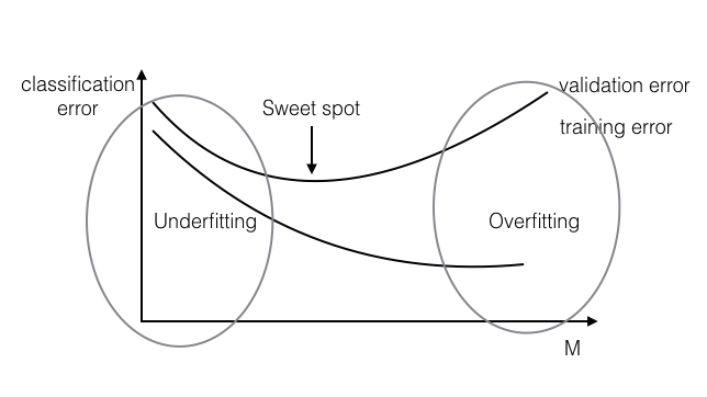
Figure 3: Early stopping