20: Neural Network
It is also known as multi-layer perceptrons and deep nets.
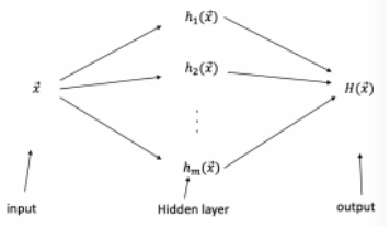
Original Problem:
How can we make linear classifiers non-linear?
$w^T+b \rightarrow w^T \Phi (x) + b$
Where Kernalization $\Phi(x)$ is a clever way to make inner products computationally tractable.
Neural network learns $\Phi:$
$\Phi(x) = \begin{bmatrix}h_1(x) \\ \vdots \\ h_m(x) \end{bmatrix}$
Each $h_i(x)$ is a linear classifier. This learns how level problem that are "simpler".
E.g. In digit classification, these detect vertical edges, round shapes, horizontals. Their output then becomes the input to the main linear classifier.
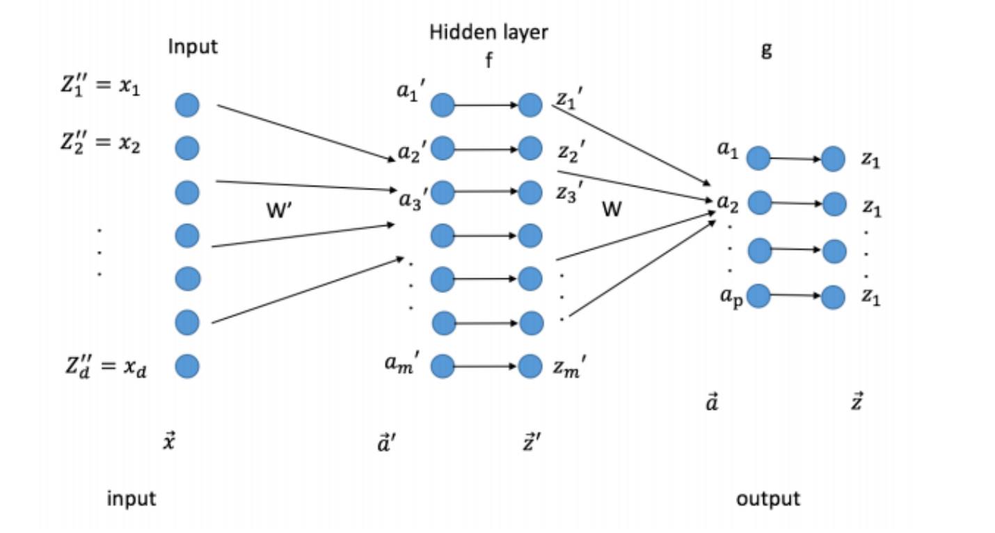
$a'_j = \sum_k w'_{jk} + b'$
$a_j = \sum_j w_{jk}z'_j + b$
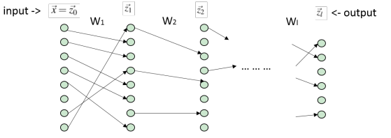
Forward Propagation:
Quiz: Try to express $vec{Z}$ in terms of $w, w', b, b', f, y$ in matrix notation
We need to learn $w, w', b, b'$. We can do so through gradien descent.
Back propagation:
Loss function for a single example: (For the entire training a set average over all training points.)
$$ L(\vec{x}, \vec{y}) = \frac{1}{2}(H(\vec{x}) - \vec{y})^2$$
Where $H(\vec{x})=\vec{z}$
$L = \frac{1}{2}(\vec{z} - \vec{y})^2$
We learn $W$ with gradient descent.
Observation (chain rule):
$\frac{\partial L}{\partial w_{ij}} = \frac{\partial L}{\partial \alpha_i} \frac{\partial \alpha_i}{\partial w_{ij}} = \frac{\partial L}{\partial \alpha_i} Z'_j$
$\frac{\partial L}{\partial w'_{jk}} = \frac{\partial L}{\partial \alpha'_j} \frac{\partial L}{\partial \alpha'_j}x_k = \frac{\partial L}{\partial \alpha'_j}Z''_k$
Let $\vec{\delta} = \frac{\partial L}{\partial \vec{\alpha}}$ and $\vec{\delta'} = \frac{\partial L}{\partial \vec{\alpha'}}$ (i.e. $\delta'_j = \frac{\partial L}{\partial \alpha_j'}$)
Gradients are easy if we know $\vec{\delta}, \vec{\delta}', \vec{\delta}'', \vec{\delta}'''$ ($\vec{\delta}'', \vec{\delta}'''$ are for deeper neural nets. )
So, what is $\delta$?
$\delta_i = \frac{\partial L}{\partial \alpha_i} = \frac{\partial L}{\partial z_i} \frac{\partial z_i}{\partial \alpha_i} = (z_i-y_i) g'(\alpha_i) = \vec{g'}(\vec{\alpha}) \circ (\vec{z} - \vec{y}) $
Note that $L = \frac{1}{2}(z_i - y_i)^2$ and $z_i = g(\alpha_i)$.
$\delta'_j = \frac{\partial L}{\partial \alpha'_j} = \sum_i \frac{\partial L}{\partial z_i} \frac{\partial z_i}{\partial \alpha_i} \frac{\partial \alpha_i}{\partial z'_j}\frac{\partial z'_j}{\partial \alpha'_j} = \sum_i \delta_i \frac{\partial \alpha_i}{\partial z'_j} \frac{\partial z'_j}{\partial \alpha'_j}$
Notet hat $\frac{\partial L}{\partial z_i} \frac{\partial z_i}{\partial \alpha_i} = \delta_i$, $\alpha=\sum_j w_{ij}z'_j + b$, and $\frac{\partial z'_j}{\partial \alpha'_j} = \delta'(\alpha'_j)$
$f'(\alpha'_j) \sum_i \delta_i W_{ij} = \vec{f'}(\vec{\alpha'}) \circ (W^T\delta)$
Typical transition functions:
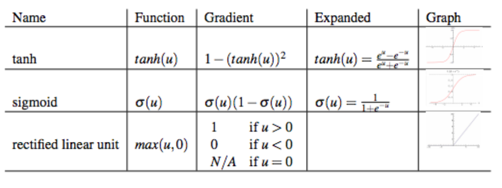
In the "Old Days", sigmoid and tanh were most popular. Nowadays, Rectified Linear Unit (Relu) are pretty fashionable.
Algorithms:
Forware Pass:
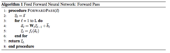
Backward Pass:
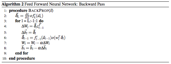
with $\vec{z_l} = f_l(\vec{a_l})$
Famous Theorem:
-ANN are univeral approximators (like SVMS, GPs, ...)
-Theoretically, a ANN with one hidden layer is as expressive as one with many hidden layers in practice if many nodes are used.
Overfitting in ANN:
Neural Networks learn lots of parameters and therefore are prone to overfitting. This is not necessarily a problem as long as you use regularization. Two popular reglarizers are the following:
- Use $l_2$ regularization on all weights (including bias terms).
- For each input (or mini-batch) randomly remove each hidden node with probability p (e.g. p=0.5) these nodes stay removed during the backprop pass, however are included again for the next input.
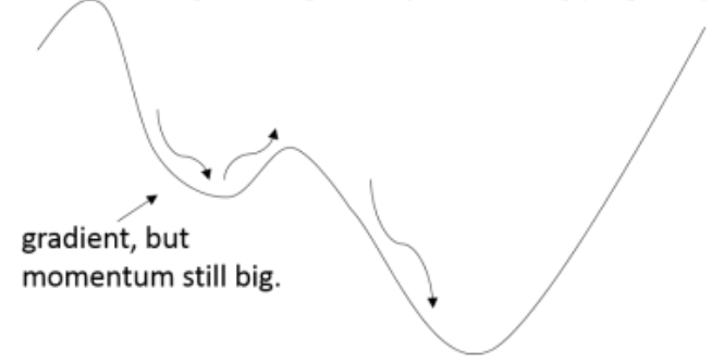
Avoidance of local minima
1. use momentum: Decline $\triangledown w_t = \Delta w_t + \mu \triangledown w_{t-1}$
$w = w- \alpha \triangledown w_t$
(i.e. still use some portion of previous gradient to keep you pushing out of small local minima.)
2. Initialize weights cleverly (not all that important)
e.g. use Autoencoders for unsupervised pre-training
3. use Relu instead of sigmoid/tanh (weights don't saturate)
Tricks and Tips
- Rescale your data so that all features are within [0,1]
- Lower learning rate
- use mini-batch (i.e. stochastic gradient descent with maybe 100 inputs at a time - make sure you shuffle inputs rnadomly first.)
- for image use convolution neural network