Project 6: Kernel SVM

"Just as we have two eyes and two feet,
duality is part of life."
--Carlos Santana

We have updated the tests for this project. Please go to Piazza resources for the latest version. The autograder is using the latest version. (November 16, 2015)

WARNING

Please start this early. The autograder takes around 20-30 minutes to run the competition. If it takes over an hour and you haven't received an email, then your code is timing out. Your code will only run for the competition if you have passed all the tests.

Files you'll edit:
`l2distance.m`	Computes the Euclidean distances between two sets of vectors. You can copy this function from previous assignments.
`computeK.m`	Computes a kernel matrix given input vectors.
`generateQP.m`	Generates all the right matrices and vectors to call the `qp` command in Octave.
`recoverBias.m`	Solves for the hyperplane bias b after the SVM dual has been solved.
`trainsvm.m`	Trains a kernel SVM on a data set and outputs a classifier.
`crossvalidate.m`	A function that uses cross validation to find the best kernel parameter and regularization constant.
`autosvm.m`	Take a look at this function. It takes as input a data set and its labels, cross validates over the hyper-parameters of your SVM and outputs a well-tuned classifier. You can "tune" this for the in-class competition.
Files you might want to look at:
`visdecision.m`	This function visualizes the decision boundary of an SVM in 2d.
`extractpars.m`	This function extracts parameters. It is a helper function for visdecision.

Introduction

In this project, you will implement a kernel SVM solver. Remember that the SVM optimization has the following dual formulation: $$ \begin{aligned} &\min_{\alpha_1,\cdots,\alpha_n}\frac{1}{2} \sum_{i,j}\alpha_i \alpha_j y_i y_j \mathbf{K}_{ij} - \sum_{i=1}^{n}\alpha_i \\ \text{s.t.} &\quad 0 \leq \alpha_i \leq C\\ &\quad \sum_{i=1}^{n} \alpha_i y_i = 0. \end{aligned} $$ This is equivalent to solving for the SVM primal $$ L(\mathbf{w},b) = C\sum_{i=1}^n \max(1-y_i(\mathbf{w}^\top\phi(\mathbf{x}_i)+b),0) + ||w||_2^2$$ where $\mathbf{w}=\sum_{i=1}^n y_i \alpha_i \phi(\mathbf{x}_i)$ and $\mathbf{K}_{ij}=k(\mathbf{x}_i,\mathbf{x}_j)=\phi(\mathbf{x}_i)^\top\phi(\mathbf{x}_j)$, for some mapping $\phi(\cdot)$. Please note that here all $\alpha_i\geq 0$. This is possible because we multiply by $y_i$ in the definition of $\mathbf{w}$. One advantage of keeping all $\alpha_i$ non-negative is that we can easily identify non-support vectors as vectors with $\alpha_i=0$.

Spiral data set

We provide you with a "spiral" data set. You can load it and visualize it with the following commands:

>> load spiral
>> whos
Variables in the current scope:

   Attr Name        Size                     Bytes  Class
   ==== ====        ====                     =====  ===== 
        xTe         2x242                     3872  double
        xTr         2x100                     1600  double
        yTe         1x242                     1936  double
        yTr         1x100                      800  double

Total is 1227 elements using 9808 bytes

>> dummy=@(X) sign(mean(X,1));
>> visdecision(xTr,yTr,dummy);

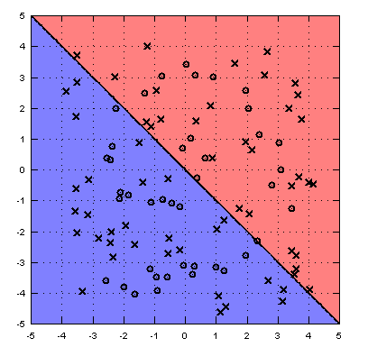
The function visdecision visualizes the data set and the decision boundary of a classifier. In this case the dummy classifier is not particularly powerful and only serves as a placeholder.

Implementing a kernelized SVM

First implement the kernel function
```
	computeK(ktype,X,Z,kpar)
```
It takes as input a kernel type (ktype) and two data sets $\mathbf{X}$ in $\mathcal{R}^{d\times n}$ and $\mathbf{Z}$ in $\mathcal{R}^{d\times m}$ and outputs a kernel matrix $\mathbf{K}\in{\mathcal{R}^{n\times m}}$. The last input, kpar specifies the kernel parameter (e.g. the inverse kernel width $\gamma$ in the RBF case or the degree $p$ in the polynomial case.)
1. For the linear kernel (ktype='linear') svm, we use $k(\mathbf{x},\mathbf{z})=x^Tz$
2. For the radial basis function kernel (ktype='rbf') svm we use $k(\mathbf{x},\mathbf{z})=\exp(-\gamma ||x-z||^2)$ (gamma is a hyperparameter, passed a the value of kpar)
3. For the polynomial kernel (ktype='poly') we use $k(\mathbf{x},\mathbf{z})=(x^Tz + 1)^p$ (p is the degree of the polymial, passed as the value of kpar)
You can use the function l2distance.m as a helperfunction.
Read through the specifications of the Octave internal quadratic programming solver, qp.
```
>> help qp
[...]
 -- Function File: [X, OBJ, INFO, LAMBDA] = qp (X0, H, q, A, b, lb, ub)
[...]
     Solve the quadratic program

          min 0.5 x'*H*x + x'*q
           x

     subject to

          A*x = b
          lb <= x <= ub

     using a null-space active-set method.
```
Here, X0 is any initial guess for your vector $\alpha$. The qp solver is not very fast (in fact it is pretty slow) but for our purposes it will do. Write the function
```
 [H,q,A,b,lb,ub]=generateQP(K,yTr,C)
 
```
which takes as input a kernel matrix K, a label vector yTr and a regularization constant C and outputs the matrices [H,q,A,b,lb,ub] so that they can be used directly with the qp solver to find a solution to the SVM dual problem. (Be careful, the b here has nothing to do with the SVM hyper-plane bias $b$.)
Implement the function
```
		[svmclassify,sv_i,alphas]=trainsvm(xTr,yTr,C,ktype,kpar);
		
```
It should use your functions computeK.m and generateQP to solve the SVM dual problem of an SVM specified by a training data set (xTr,yTr), a regularization parameter (C), a kernel type (ktype) and kernel parameter (kpar). For now ignore the first output svmclassify (you can keep the pre-defined solution that generates random labels) but make sure that sv_i corresponds to all the support vectors (up to numerical accuracy) and alphas returns an n-dimensional vector of alphas.
Now that you can solve the dual correctly, you should have the values for $\alpha_i$. But you are not done yet. You still need to be able to classify new test points. Remember from class that $h(\mathbf{x})=\sum_{i=1}^n \alpha_i y_i k(\mathbf{x}_i,\mathbf{x})+b$. We need to obtain $b$. It is easy to show (and omitted here) that if $C>\alpha_i>0$ (with strict $>$), then we must have that $y_i(\mathbf{w}^\top \phi(\mathbf{x}_i)+b)=1$. Rephrase this equality in terms of $\alpha_i$ and solve for $b$. Implement
```
		bias=recoverBias(K,yTr,alphas,C);
		
```
where bias is the hyperplane bias $b$ (Hint: This is most stable if you pick an $\alpha_i$ that is furthest from $C$ and $0$. )
With the recoverBias function in place, you can now finish your function trainsvm.m and implement the remaining output, which returns an actual classifier svmclassify. This function should take a set of inputs of dimensions $d\times m$ as input and output predictions ($1\times m$). You can evaluate it and see if you can match my testing and training error exactly:
```
>> load spiral
>> svmclassify=trainsvm(xTr,yTr,6,'rbf',0.25);
Generate Kernel ...
Generate QP ...
Solve QP ...
Recovering bias ...
Extracting support vectors ...
>> testerr=sum(sign(svmclassify(xTe))~=yTe(:))/length(yTe)
testerr =  0.29339
>> trainerr=sum(sign(svmclassify(xTr))~=yTr(:))/length(yTr)
trainerr = 0.13000
```
If you play around with your new SVM solver, you will notice that it is rather sensitive to the kernel and regularization parameters. You therefore need to implement a function
```
[bestC,bestP,bestvalerror]=crossvalidate(xTr,yTr,ktype,Cs,kpars)
```
to automatically sweep over different values of C and kpars and output the best setting on a validation set (xTv,yTv). For example you could set Cs=2.^[-5:5] to try out different orders of magnitude. Cut off a section of your training data to generate a valication set.

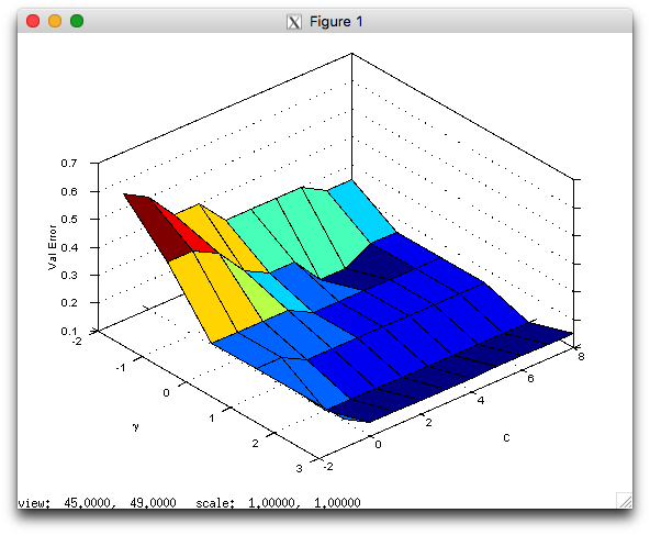
If you did everything correctly, you should now be able to visualize your cross validation map:
```
>> load spiral
>> [bestC,bestP,bestval,allerrs]=crossvalidate(xTr,yTr,'rbf',2.^[-1:8],2.^[-2:3]);
>> [xx,yy]=meshgrid(-2:3,-1:8);
>> surf(xx,yy,allerrs);
>> xlabel('\gamma'); ylabel('C'); zlabel('Val Error');
```
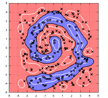
The result should look similar to this image: You can now also take the best parameters and train your SVM. The following code trains the SVM with crass validated parameters, computes the test error and visualizes its decision boundary.
```
>> svmclassify=trainsvm(xTr,yTr,bestC,'rbf',bestP);
>> testerr=sum(sign(svmclassify(xTe))~=yTe(:))/length(yTe)
testerr =  0.15289
>> visdecision(xTe,yTe,svmclassify,'vismargin',true);
```

Extra Credit

Implement the function autosvm.m. Currently it takes a data set as input and tunes the hyper-parameters for the RBF kernel to perform best on a hold-out set (with your crossvalidation.m function). Can you improve it? (For example, you may look into adding new kernels to computeK.m, use telescopic cross validation, or use k-fold cross validation instead of a single validation set.)

Hints

It helps if you execute

>> more off

whenever you start or Octave console, to see the output of your functions on the screen right away.