CS4620 Assignment 6: Shaders
Overview
In this assignment, you will implement some shaders in GLSL, a graphics-specific language that lets you write programs that run on the graphics processor (GPU).
The framework code for this asignment is in the assignment6 repository. There are three components to the assignment:
- Implement a microfacet shader in microfacet.html.
- Implement specular (mirror-like) reflection under environment lighting in environment.html.
- Implement a normal mapping shader (without environment mapping) in normal.html.
The implementation of each part is contained in its own webpage, which includes a framework based on the mesh viewer we used in lecture. This will allow you to load any meshes and textures you might like to test with. For this assignment, the Javascript code that sets up the scene is provided, so you only have to implement the shaders themselves, but be sure to understand what uniforms and attributes are being passed to your GLSL program. Some of the uniforms may be controlled using sliders on the webpage.
The framework is a simple single-page application built on the popular Three.js 3D graphics library. Although in principle you don't need to worry about how this application works, you might like to read the fundamentals article from the tutorial site threejsfundamentals.org to get oriented to this system, then look around the code (much of which is in js/A6Common.js. Our framework loads meshes into a simple scene graph with some lights and a camera and applies a THREE.ShaderMaterial to the mesh. This material allows us to provide a vertex shader and a fragment shader to be used for rendering the mesh. Three.js defines some uniforms and some attributes that your shaders need to use; they are documented here but also repeated in comments in the starter code.
The shaders are in script tags embedded in the HTML documents themselves. You will edit and submit these directly. We have marked all the shaders you need to write with TODO#A6 in the source code.
The easiest way to run the applications is to run a web server in the assignment directory with python -m http.server (using the same Python 3 installation you used for the imaging and ray tracing assignments), and then load the pages from http://localhost:8000. Depending on your browser you may also be able to load some using file:// URLs. As you work on your code you will need to reload the page after each change, and you'll see any errors (including compilation errors in your GLSL code) in the browser's console.
A few test meshes and textures have been provided in the data directory.
Example: Phong Shader
We have provided an example in phong.html. You do not need to modify this file, but it may be useful as a reference. Note the built-in uniforms and attributes provided by Three.js as well those we have provided via Javascript. Uniforms include the model, view, and projection matrices. Attributes include vertex positions and normals (in local object space). See also how the "Roughness" slider changes the roughness uniform with a corresponding change in the rendering. (The slider adjusts the reciprocal of the Phong exponent; we have chosen to display it this way so that moving the slider to the right has a similar effect to doing the same with the microfacet shader.)
Also note how the lights are handled. There is one uniform array for the positions and another for the colors. The constant NUM_LIGHTS gives the number of lights. There is also ambient lighting that works just like in the ray tracer, except that it's set by a separate variable rather than an entry in the list of lights, and the material's ambient color is equal to the diffuse reflectance.
Note how this shader determines the diffuse color based on the Boolean uniform hasTexture. When this is true it looks up in diffuseTexture and otherwise it just uses diffuseReflectance. The values stored in the texture are diffuse reflectance, rather than diffuse coefficient, so they need to be divided by \(\pi\) to get the diffuse coefficient.
Finally, note that this example performs the bulk of its computations in eye space, as this is the most convenient for the provided set of built-in uniforms. We recommend you do the same. Similarly, while we have provided a toggle between fixing light positions to world space and fixing light positions to eye space, in the shader the light position uniforms will always be provided in eye space.
Problem 1: Microfacet Shader
The Blinn-Phong shading implemented in the example shader gives OK results—but it's far from the reality of light reflection. For more realistic appearance, we should use more sophisticated models, such as those based on the widely-used microfacet framework.
You will implement a microfacet-based lighting model that includes diffuse reflection and also models light that reflects specularly from the top surface of the material. The microfacet model you're required to implement uses the Beckmann distribution to model the roughness of the surface. You are supposed to implement the overall fragment shader, but we are providing implementations of the \(F\), \(D\), and \(G\) functions below to save you the effort of typing in the long formulas that define them.
This model is defined in terms of a bidirectional reflectance distribution function (BRDF). The BRDF is simply the function of normal, viewing direction, and light direction that describes how the surface reflects light; it is multiplied by the irradiance from the source to compute the reflected light. For a diffuse surface the BRDF is just the diffuse coefficient \(k_d = R_d/\pi\), and for models that include specular reflection, like the Modified Blinn-Phong model we saw earlier, the BRDF is the sum of a diffuse BRDF and a specular one that is not constant. With a diffuse reflectance \(R_d\) and a specular BRDF \(f_r\), the shading equation for a single light source is as follows: \[\left(\frac{R_d}{\pi} + f_r(\omega_i, \omega_o, n)\right) \frac{I_l\max ( n \cdot \omega_i , 0 )}{r^2} \]
- \(\omega_i\): Direction unit vector along incoming ray.
- \(\omega_o\): Direction unit vector along outgoing ray.
- \(n\): unit normal vector of surface at the shaded point.
- \(I_l\): intensity of light source.
- \(r\): distance to light source.
These computations should be repeated for each visible light in the scene and the contributions summed.
The term in parentheses is the full BRDF of the surface, including the Lambertian BRDF (which is a constant, since diffuse reflection sends light equally in all directions) and the specular BRDF \(f_r\). The value of function \(f_r(\omega_i, \omega_o, n)\) here is a scalar so it adds to all three components of the RGB diffuse color. \(I_l\) is the color of the light in the lightColors array. You will need to look up the diffuse reflectance \(R_d\) in the texture provided in the diffuseTexture uniform, which you can do using the texture2D function that is built into GLSL. The specific microfacet model we use comes from this paper and is the product of several factors: \[ f_r(\omega_i,\omega_o,n) \; = \; \frac{F(\omega_i,h)G(\omega_i,\omega_o,h)D(h)}{4|\omega_i \cdot n| |\omega_o \cdot n|} \]- \(h\): normalized half vector of \(\omega_i\) and \(\omega_o\): \[ h(\omega_i, \omega_o) \; = \; \frac{\omega_i + \omega_o}{|\omega_i + \omega_o|} \]
- \(F(\omega_i,h)\): This is the Fresnel reflection factor for unpolarized light. It is implemented in the provided function ufacetF.
- \(D(h)\): This factor is the microfacet distribution function; we use the Beckmann distribution. It is implemented in the provided function ufacetD.
- \(G(\omega_i,\omega_o,h)\): This is the Smith shadowing-masking term; it is designed based on the choice of microfacet distribution function \(D(h)\). For the Beckmann model, we use a rational approximation calculated by Walter et al. It is implemented in the provided function ufacetG.
Implement the shading equation in fragmentShader in microfacet.html. Use vertexShader to pass any data you will need to the fragment shader. Handle light sources, textures, and ambient lighting in the same way as the Phong shader example.
Because the highlights from point lights are really bright, they tend to look overly clipped with linear tone mapping, and it is difficult to get light colored surfaces to look good. Just as we did with our digital photograph in the imaging assignment, we'll apply the ACES filmic tone mapping curve to this shading to make a more pleasing image. You'll find the same ACES_filmic that we used in that assignment in the framework code for your use. Don't forget to apply the exposure (before tone mapping) and gamma correction (after tone mapping). (We feel compelled to mention that this ought to be done on the whole image as a post-process, but it's basically equivalent in this case since there is basically nothing else in the image other than what is produced by your shader.)
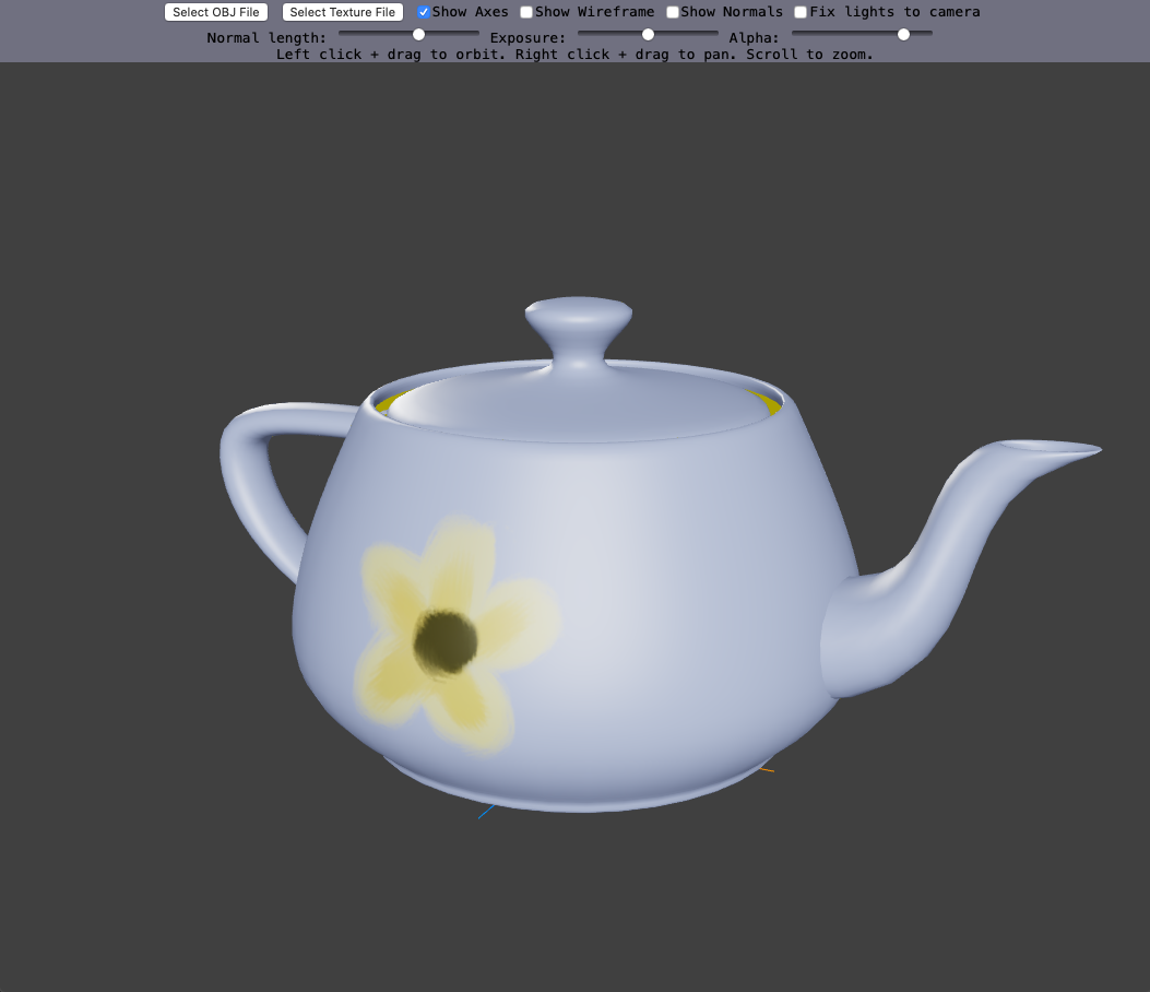
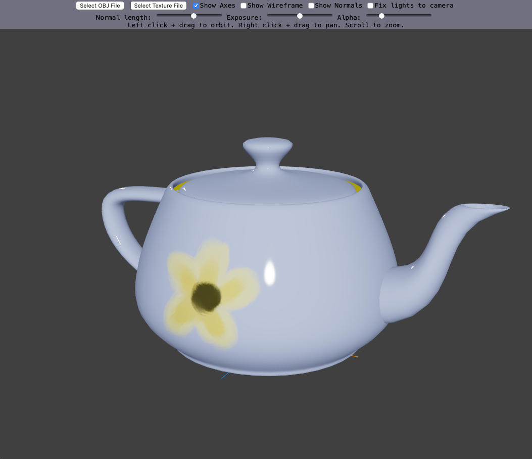
You can test your implementation on this model and texture:
- Mesh: data/meshes/teapot.obj; texture: data/textures/Flower.png
The left image in the above uses the default alpha value, while the right image has alpha set much lower to achieve a sharper and brighter specular reflection. The exposure is set to the default (0).
Problem 2: Environment Mapping
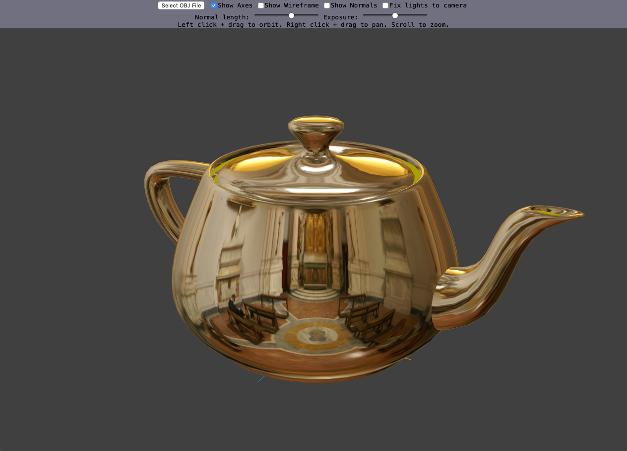
You used point lights in the Raytracer and Scene assignments. Real world scenes usually have much more complex lighting conditions than that and environment mapping is a clever technique to capture complex lighting in a texture. The idea of an environment map is that the illumination from the environment depends on which direction you look, and an environment map is simply a texture you look up by direction to answer the question "how much light do we see if we look in that direction?". Your task here is to implement specular reflection under a given environment map.
In OpenGL, there is a special kind of texture called a cube map, which stores images of the distant environment. A cube map consists of six faces, and each of them has a 2D texture that shows the environment viewed in perspective through one face of the cube. You can sample a cubemap with a 3D vector in order to get environment light intensity in the direction that vector is pointing. See section 11.2 and 11.4.5 of the book.
In this assignment we have already loaded a cubemap for you as the uniform environmentMap, of type samplerCube. Similarly to a 2D texture, you can look up into a cube using the textureCube function that is built into GLSL, except the argument you pass is a direction vector rather than a 2D texture coordinate.
Your task is to implement specular reflection under environment lighting. Given a viewing direction and a normal direction, we can compute the direction of a mirror reflection (see slides from class), and then use it to sample the cube map. You may assume the environment map is fixed in eye space; i.e. the mouse rotates the scene relative to the environment map, but the environment map remains fixed relative to the camera. Implement the vertexShader and fragmentShader in environment.html.
Problem 3: Normal Mapping
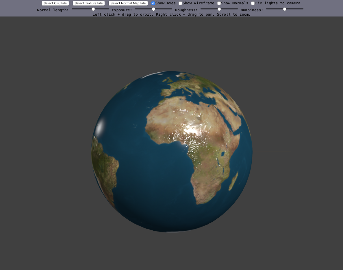
Creating detailed models with thousands of polygons is a time consuming job and rendering them in real-time can be also problematic. However, with normal mapping, we can make simple, low resolution models look like highly detailed ones. In addition to the polygon model, we provide a high resolution normal map which we can use in the fragment shader instead of the interpolated normals, adding detail to the low resolution model. Normal maps can be generated procedurally in the shaders or read from an image and used as a texture.
Your task is to implement normal mapping in normal.html. You should use a shading model just like the provided Phong shading example, including its exposure and ambient term. But instead of using the mesh's (interpolated) normal, you will need to use a weighted combination of the normal and two tangent vectors. These are provided to the vertex shader as attributes: normal (as before), tangent, and tangent2. These three vectors form a right-handed orthonormal basis, where tangent is perpendicular to normal and points towards the increasing \(u\) direction of the UV coordinates, and normal2 completes the basis by being perpendicular to the other two. In addition we have provided a bumpiness uniform as a crude way of scaling the "strength" of the normal map. All-in-all, the resulting normal should be proportional to the sum of the following:
- tangent times (the red channel of the normal map texture - 0.5) times bumpiness.
- tangent2 times (the green channel of the normal map texture - 0.5) times bumpiness.
- normal times (the blue channel of the normal map texture - 0.5).
We subtract 0.5 from each channel since color channel values run from 0 to 1, but we want to be able to represent directions with negative components.
Note that you will need to pass (and implicitly interpolate) normal, tangent, and tangent2 between the vertex and fragment shaders. You can do this by using varyings.
You can test your implementation on this model and normal map:
- Map of the Earth: mesh: data/meshes/sphere.obj; texture: data/textures/earthmap1k.jpg; normal map: data/textures/earthNormalMap_1k.png
What to Submit
Submit a zip file containing your solution organized the same way as the code on Github. Include a README in your zip that contains:
- You and your partner's names and NetIDs.
- Any problems with your solution.
- Anything else you want us to know.