April 16, 1999
Stats: Min: 21, Max: 88, Mean: 53.8, Std.Dev: 16.8
Prelim 2
April 16, 1999
Stats: Min: 21, Max: 88, Mean: 53.8, Std.Dev: 16.8
| (a) | true | Live variable analysis is a backward data-flow analysis. |
| (b) | false | When a valid, non-spilling register allocation exists, a graph-coloring register allocator always finds it. |
| (c) | true | The most permissive safe subtyping rules treat immutable and mutable fields of records differently. |
| (d) | false | The problem of finding the optimum tiling of an IR tree based on the sum of costs of instructions selected is NP-complete. |
| (e) | true | A loop in the control flow graph may contain more than one back edge. |
| (f) | true | Copy propagation analysis is a forward data-flow analysis which propagates sets of available expressions that are variables. |
| (g) | true | In canonical IR trees, every side-effect to a temporary is found in a distinct statement node. |
| (h) | false | The consecutive instructions mov ax, [bx + 12] and mov [cx + 4], dx may be interchanged. |
| (i) | true | In an anti-dependency between two instructions, the later instruction writes to a location that the earlier one reads. |
| (j) | false | Loads from memory location should be scheduled as close as possible to their uses. |
| (k) | false | The register interference graph contains information about instruction dependencies. |
| (l) | true | In C++ implementations, objects may contain pointers to multiple dispatch vectors. |
In an object-oriented language such as Java that supports multiple supertypes (interfaces may implement multiple interfaces), a sparse dispatch vector technique may be used to avoid the conflicts that arise when assigning method indices sequentially. Rather than allocating method indices sequentially, a global phase of method index computation is performed, allocating indices to methods in such a way that if a dispatch vector contains methods A and B, their method indices are always different. A simple algorithm for index allocation is to give every method in the entire class hierarchy a different method index, but this approach can waste a great deal of memory because many dispatch vector slots will be empty. It also will hurt data-cache performance. A better algorithm is needed.
Assuming that we have available a list of the methods supported by each class in the class hierarchy, the problem of finding the optimum allocation of method indices is NP-complete. However, we can assign method indices in a way that usually reuses dispatch vector entries effectively. Sketch in moderate detail an efficient algorithm for method index allocation.
Apply graph coloring to this problem as follows:
Create a graph in which each distinct method is a node. Place an edge between every pair of nodes whose methods appear in the same class, either through definition in that class, or through inheritance from some superclass. Color the graph, drawing from an unbounded number of colors. Each color represents a method index. Preferentially choose nodes with the lowest number of conflicts at each stage, and break ties by choosing nodes that occur in the fewest classes. Since dispatch vectors may be unbounded in size, there is never any need to "spill" a method. This algorithm will reproduce the compact index assignment of the standard dispatch vector layout when the hierarchy only contains single supertypes, but will reuse dispatch vector slots fairly effectively.
Every method call and field reference (except through "this") require run-time verification that the object is not pointing to null. The result of such a check in Java is a NullPointerException (when a null pointer is in fact dereferenced). A C program has no such checks (and therefore you may get segmentation violations instead).
An alternative to allowing null pointers is to support maybes. A value of type maybe(T) is either full (it represents a value of type T), or is empty (it contains no value, corresponding to a null pointer). An expression of type maybe(T) may be used wherever an expression of type T may be used; however, if at run time the maybe is empty, the program aborts. The advantage of having maybes is that when the compiler sees an expression whose declared type is T, it knows that the expression cannot evaluate to a null pointer. The type maybe(T) supports one operation in addition to all of the operations of values of type T: the built-in function empty() may be invoked on values of type maybe(T) to obtain a boolean indicating whether the maybe contains a value. For example, a singly linked list might be implemented in Iota+ by using maybes as follows:
class List {
    head: object
    tail: maybe(List)
    length(): int = {
        n: maybe(List) = tail;
        c: int = 0;
        while (!empty(n)) { c++; n = n.tail; }
    }
    …
}
T[empty(E)] = BINOP (=, T[E], 0)
maybe(T)
makes less sense for primitive types T or for T = maybe(T'). It can be made to work by
boxing primitive types and maybes up into objects, however.
There are actually three different rules needed to type check maybes. We gave credit for providing either of the rules dealing with subtyping.
| A |- E : maybe(T) | A |- T £ object | A |- S £ T | ||
| A |- empty(E) : bool | A |- maybe(T) £ T | A |- maybe(S) £ maybe(T) |
L0: x = y + x
    w = 2 * x
    if s == u goto L1 else goto L4
L1: s = w + 1
L2: y = s + x
    if y > 1000 goto L0 else goto L3
L4: x = w + u
    u = u – 1
    goto L2
L3:
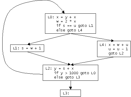
| Instruction | n | def(n) | use(n) | succ(n) | in[n] | out[n] |
|---|---|---|---|---|---|---|
| L0: x = y + x | 1 | {x} | {x, y} | {2} | {x, y, s, u} | {s, x, u} |
| w = 2 * x | 2 | {w} | {x} | {3} | {s, x, u} | {s, u, w, x} |
| if s == u goto L1 else goto L4 |
3 | {} | {s, u} | {4, 7} | {s, u, w, x} | {w, x, u, s} |
| L1: s = w + 1 | 4 | {s} | {w} | {5} | {w, x, u} | {s, x, u} |
| L2: y = s + x | 5 | {y} | {s, x} | {6} | {s, x, u} | {y, s, x, u} |
| if y > 1000 goto L0 else goto L3 |
6 | {} | {y} | {1, 10} | {y, s, x, u} | {y, s, x, u} |
| L4: x = w + u | 7 | {x} | {w, u} | {8} | {w, u, s} | {s, x, u} |
| u = u - 1 | 8 | {u} | {u} | {9} | {s, x, u} | {s, x, u} |
| goto L2 | 9 | {} | {} | {5} | {s, x, u} | {s, x, u} |
| L3: | 10 | {} | {} | {} | {s, u} |
Live-variable analysis (Appel, p.225) is a backwards data-flow analysis (in contrast to the forward data-flow analysis in HW3); the most common mistake was not properly defining a meet operator and a flow function:
out[n] = /\ (over all pi in successors(n), in[pi]) = U (pi in successors(n), in[pi])
in[n] = F (out[n]) = use[n] U { out[n] - def[n] }
People tended to determine liveness by inspection (and then it appeared as if the inspection were being done in a forward direction), to associate liveness with edges in the control flow graph (implicitly assuming that in == out), or to determine liveness for basic blocks rather than for each individual statement. This is an important distinction to keep in mind: basic blocks describe the flow of control through the program. Live-variable analysis needs to be done on a statement-by-statement basis, because the liveness of a variable may change within a basic block.
A second small mistake was to correctly determine liveness upon entry and exit from each node by associating the variable sets with edges, but then to neglect to take the union of sets over all entry and exit edges to yield the live-in and live-out sets at each node.
L1: if b goto L2 else goto L3
L2: x = a + b
    a = 10
    goto L4
L3: y = a + b
    b = y
L4:
Since the expression b OP c will be evaluated no matter which path is taken by the program, we can hoist the computation of b OP c to the very busy point p and store the result in a variable. Subsequent computation of b OP c (before any assignment to b or c) can simply be replaced by the variable. Hence, the identification of very busy expressions enable us to optimize programs in two ways: (i) the size of the resulting program is smaller and (ii) the running time of the program is smaller because we avoid redoing work.
This is a backward analysis. By definition of "very busy expressions", an expression (y OP z) is very busy at a point p if it is evaluated on every path from p before some assignment to y or z. Hence, the problem of determining whether y OP z is very busy at p is equivalent to the problem of checking whether the same expression is evaluated by every successor of p. It is obvious from the backward flow of information that this is a backward analysis.
To set up the data-flow equations for solving very busy expressions, we first define the gen and kill sets for all kinds of quadruples. Since the problem is to identify very busy expressions, both gen and kill are sets of expressions in the program, with gen[n] containing the set of expressions generated by quadruple n and kill[n] containing the set of expressions killed by n. It turns out that the gen and kill sets for computing very busy expressions are exactly the same as those for computing available expressions. (Refer to Table 17.4, p.394 of Appel for details.)
With gen and kill properly defined, we can set up the the data-flow equations in a straightforward manner:
in[n] = gen[n] È (out[n] - kill[n])
out[n] = Ç i in succ[n] in[i]
From (c), out[n] = intersection of in[i] for all i in succ[n]. Hence, if there exists a j in succ[n] such that j is unreachable in all executions of the programs (in other words, j is dead code), the above equations would underestimate out[n] and hence the set of very busy expressions at point n. Any example conveying this idea will be awarded full credit. For a concrete example, consider the code example given in the question. Set b to true and delete the statement y = a + b in L3. In this case, the basic block L3 becomes dead code. Ideally we would still want to say that a + b is a very busy expression at L1, but since there is no efficient way to tell exactly which paths are real and which are not, we are forced to accept the solution returned by the data-flow analysis, which says that a + b is not very busy at L1.
By now you should have realized that there are strong similarities among the various data-flow problems. The data-flow equations we have seen so far can be distinguished by:
We can in fact classify various data-flow problems seen in class along these two
dimensions:
| all paths | any path | |
|---|---|---|
| forward | available expressions | reaching definitions |
| backward | very busy expressions | live variables |