 Data Assumption: \(y_{i} \in \mathbb{R}\)
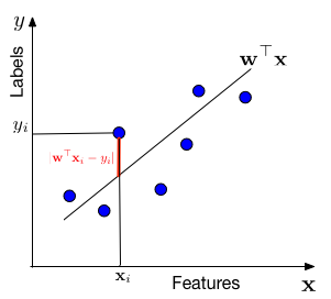
In words, we assume that the data is drawn from a "line" \(\mathbf{w}^\top \mathbf{x}\) through the origin (one can always add a bias / offset through an additional dimension, similar to the Perceptron). For each data point with features \(\mathbf{x}_i\), the label \(y\) is drawn from a Gaussian with mean \(\mathbf{w}^\top \mathbf{x}_i\) and variance \(\sigma^2\). Our task is to estimate the slope \(\mathbf{w}\) from the data.
We are minimizing a loss function, \(l(\mathbf{w}) = \frac{1}{n}\sum_{i=1}^n (\mathbf{x}_i^\top\mathbf{w}-y_i)^2\). This particular loss function is also known as the squared loss. Linear regression is also known as Ordinary Least Squares (OLS). OLS can be optimized with gradient descent or Newton's method.
This objective is known as Ridge Regression.
In general, we want to solve the following optimization problem: $$ \min_{\mathbf{w}} \frac{1}{n}\sum_{i=1}^n (\mathbf{x}_i^\top\mathbf{w}-y_i)^2 + \lambda \|\mathbf{w}\|_2^2 $$ where \(\lambda \geq 0\) is a regularization parameter. When \(\lambda = 0\), we recover Ordinary Least Squares. When \(\lambda > 0\), we have Ridge Regression.
To find the optimal \(\mathbf{w}\), we compute the gradient of the objective function with respect to \(\mathbf{w}\). Using matrix notation where \(\mathbf{X} = [\mathbf{x}_1, \ldots, \mathbf{x}_n]\) and \(\mathbf{y} = [y_1, \ldots, y_n]\), we can rewrite the objective as: $$ L(\mathbf{w}) = \frac{1}{n}(\mathbf{X}^\top\mathbf{w} - \mathbf{y}^\top)^\top(\mathbf{X}^\top\mathbf{w} - \mathbf{y}^\top) + \lambda \mathbf{w}^\top\mathbf{w} $$
Taking the gradient: $$ \nabla_{\mathbf{w}} L(\mathbf{w}) = \frac{2}{n}\mathbf{X}(\mathbf{X}^\top\mathbf{w} - \mathbf{y}^\top) + 2\lambda\mathbf{w} $$
At the optimum, the gradient must be zero. Setting \(\nabla_{\mathbf{w}} L(\mathbf{w}) = \mathbf{0}\) and rearranging: $$ (\mathbf{X}\mathbf{X}^\top + n\lambda\mathbf{I})\mathbf{w} = \mathbf{X}\mathbf{y}^\top $$ This is a system of linear equations that we need to solve for \(\mathbf{w}\).
The nature of the solution depends on \(\lambda\) and the rank of \(\mathbf{X}\):
Case 1: \(\lambda > 0\) (Ridge Regression)
The matrix \(\mathbf{X}\mathbf{X}^\top + n\lambda\mathbf{I}\) is always invertible because adding \(n\lambda\mathbf{I}\) (with \(\lambda > 0\)) makes the matrix strictly positive definite. This guarantees a unique solution regardless of the rank of \(\mathbf{X}\).
Case 2: \(\lambda = 0\) and \(\mathbf{X}\) has full rank (Ordinary Least Squares, overdetermined)
If \(\mathbf{X}\) has full row rank (i.e., \(\text{rank}(\mathbf{X}) = d\) where \(d\) is the number of features and \(d \leq n\)), then \(\mathbf{X}\mathbf{X}^\top\) is invertible. This also gives a unique solution. This typically occurs when we have more data points than features (\(n \geq d\)) and the data points span the entire feature space.
Case 3: \(\lambda = 0\) and \(\mathbf{X}\) does not have full rank (Ordinary Least Squares, underdetermined)
If \(\text{rank}(\mathbf{X}) < d\), then \(\mathbf{X}\mathbf{X}^\top\) is not invertible. This occurs when we have fewer data points than features (\(n < d\)) or when the data points do not span the entire feature space (e.g., they lie in a lower-dimensional subspace). In this case, there are infinitely many solutions that all achieve the same minimum loss.
When a unique solution (cases 1 and 2) exists, it can be written as: $$ \mathbf{w}^* = (\mathbf{X}\mathbf{X}^\top + n\lambda\mathbf{I})^{-1}\mathbf{X}\mathbf{y}^\top $$ For \(\lambda = 0\) (assuming full rank), this simplifies to: $$ \mathbf{w}^* = (\mathbf{X}\mathbf{X}^\top)^{-1}\mathbf{X}\mathbf{y}^\top $$
When \(\mathbf{X}\) does not have full rank and the linear equations are underdetermined (case 3), the solution set forms an affine subspace. To understand this, we decompose any weight vector \(\mathbf{w}\) into two orthogonal components: $$ \mathbf{w} = \mathbf{w}_{\parallel} + \mathbf{w}_{\perp} $$ where:
A key observation: the loss function depends only on \(\mathbf{w}_{\parallel}\)! This is because: $$ \mathbf{x}_i^\top\mathbf{w} = \mathbf{x}_i^\top(\mathbf{w}_{\parallel} + \mathbf{w}_{\perp}) = \mathbf{x}_i^\top\mathbf{w}_{\parallel} + \mathbf{x}_i^\top\mathbf{w}_{\perp} = \mathbf{x}_i^\top\mathbf{w}_{\parallel} $$ since \(\mathbf{x}_i^\top\mathbf{w}_{\perp} = 0\) (as \(\mathbf{w}_{\perp}\) is in the null space of \(\mathbf{X}^\top\)).
Therefore, any two weight vectors with the same \(\mathbf{w}_{\parallel}\) component achieve the same loss, regardless of their \(\mathbf{w}_{\perp}\) component. The solution set is: $$ \{\mathbf{w}^*_{\parallel} + \mathbf{w}_{\perp} : \mathbf{w}_{\perp} \in \text{null}(\mathbf{X}^\top)\} $$ where \(\mathbf{w}^*_{\parallel}\) is any particular solution to the linear system.
Among all solutions that minimize the loss, there is one with the smallest \(\ell_2\) norm. This is called the minimum-norm solution, and it is the unique solution where \(\mathbf{w}_{\perp} = \mathbf{0}\), i.e., the solution that lies entirely in the column space of \(\mathbf{X}\).
The minimum-norm solution can be computed using the Moore-Penrose pseudoinverse: $$ \mathbf{w}^*_{\text{min-norm}} = \mathbf{X}^\top(\mathbf{X}\mathbf{X}^\top)^{\dagger}\mathbf{y}^\top $$ where \((\mathbf{X}\mathbf{X}^\top)^{\dagger}\) denotes the pseudoinverse of \(\mathbf{X}\mathbf{X}^\top\).
Instead of solving the linear system directly, we can use gradient descent. Starting from an initial guess \(\mathbf{w}^{(0)}\), we repeatedly update with \(\eta = 0\) is the learning rate (step size): $$ \mathbf{w}^{(t+1)} = \mathbf{w}^{(t)} - \eta \left[\frac{2}{n}\mathbf{X}(\mathbf{X}^\top\mathbf{w}^{(t)} - \mathbf{y}^\top) + 2\lambda\mathbf{w}^{(t)}\right] $$
For large datasets, computing the full gradient over all \(n\) samples can be expensive. Stochastic Gradient Descent approximates the gradient using a single randomly selected data point (or a small batch). At iteration \(t\), we randomly sample an index \(i\) and update: $$ \mathbf{w}^{(t+1)} = \mathbf{w}^{(t)} - \eta \left[2\mathbf{x}_i(\mathbf{x}_i^\top\mathbf{w}^{(t)} - y_i) + 2\lambda\mathbf{w}^{(t)}\right] $$
An important property of gradient descent (and SGD) is what solution it converges to in the underdetermined case (\(\lambda = 0\) and \(\mathbf{X}\) not full rank).
Key Result: If gradient descent is initialized at \(\mathbf{w}^{(0)} = \mathbf{0}\) (or any point in the column space of \(\mathbf{X}\)), then if it converges, it converges to the minimum-norm solution. More generally, if initialized at any \(\mathbf{w}^{(0)} = \mathbf{w}^{(0)}_{\parallel} + \mathbf{w}^{(0)}_{\perp}\), gradient descent converges to the solution whose null space component equals \(\mathbf{w}^{(0)}_{\perp}\).
The reason for this behavior is that the gradient is always in the column space of \(\mathbf{X}\), i.e. the span of the features. This is very easy to see in the case of SGD, where update is always proportional to a data point: $$\mathbf{w}^{(t+1)} = \mathbf{w}^{(t)} - \eta \left[2\mathbf{x}_i(\mathbf{x}_i^\top\mathbf{w}^{(t)} - y_i)\right] .$$ More generally, the gradient is: $$ \nabla_{\mathbf{w}} L(\mathbf{w}) = \frac{2}{n}\mathbf{X}(\mathbf{X}^\top\mathbf{w} - \mathbf{y}^\top) $$ This is a linear combination of the columns of \(\mathbf{X}\), so it lies in the column space of \(\mathbf{X}\).
Therefore, each gradient descent update only changes \(\mathbf{w}\) by a vector in the column space of \(\mathbf{X}\). This means:
This explains the implicit bias of gradient descent: when initialized at the origin, it finds the minimum-norm solution among all solutions that minimize the training loss. This implicit regularization is one reason why gradient descent can generalize well even in overparameterized models.