
%%%%%%%% Plot the coordinates and contact matrix  %%%%%%%%

coorCA = pickCA('1LAP.pdb');                    % Extract the CA coordinates
%plot3(coorCA(:,1), coorCA(:,2), coorCA(:,3));  % Plot the CA coordinates
make_contmap(coorCA);                           % Create and plot the contact map


%%%%%%%% Analyze distances between representations %%%%%%%

coorN = pickN('1LAP.pdb');          % Retrieve the N coordinates
dist1 = norm(coorCA - coorN)        % Compute and output distance between coorCA and coorN

origCA = trans_origin(coorCA);      % Re-center the CA coordinates at 0.
origN  = trans_origin(coorN);       % Re-center the N  coordinates at 0.
dist2  = norm(origCA - origN)       % Output distance between re-centered matrices

%%%%%%%%%%%%%%%%%%%%%%%%%%%%%%%%%%%%%%%%%%%%%%%%%%%%%%%%%%
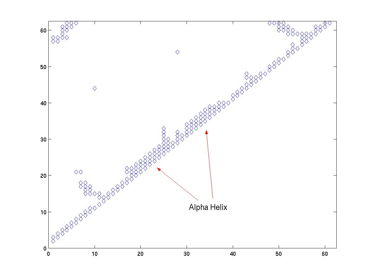
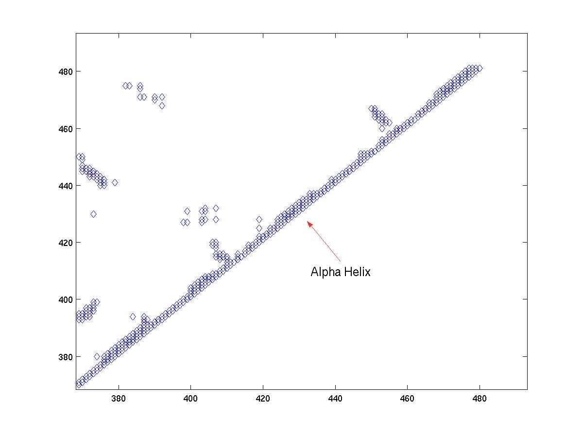
Once we have zoomed in on a region of the main diagonal, we can proceed to identify the structural elements. Alpha helices are compact structures, where several neighboring amino acids are packed close together. Therefore, in an alpha helix, we expect the alpha carbon i to have at least four contacts: i + 1, ..., i + 4. If we see a region along the main diagonal where position i has 4 or more contacts for several consequtive values of i, then that region indicates an alpha-helix. For example, see Figure 3a and Figure 3c.
One the other hand, Beta-Sheet strands are fairly spread-out structures, and so we don't
expect their alpha-carbons to be packed closely. In a typical strand, each amino acid will have
one or two contacts. In addition, when strands run parallel to one another in a beta-sheet
structure, amino acids can wind up having contacts in remote positions, as illustrated below.
dist1 =

   19.5119

dist2 =

   19.5069
As we can see, the distance between the CA and N representation has not decreased significantly, even though we translated both coordinate matrices to the origin. In order to decrease the distance further, we would need to rotate on the coordinate matrices until it overlaps the other.