Programs and functions

While using MATLAB as a fancy calculator has its own advantages, it is also possible to use MATLAB as a programming language and to develop with it significant programs with considerable ease.

Files that end with .m are recognized as MATLAB programs (or functions) and can be executed in MATLAB by typing their name. For example, the text below is kept in a file plotlog.m

% plot log(x) versus x

x = linspace(1,10);

y = log(x);

plot(x,y)

The first line is a comment in the file that tells us what the program is all about (it is plotting the log function) In the first line we assign to the array x 100 points between 1 and 10. The second line computes the log(x) (natural logarithm) and the third line plots x versus y.

To execute this program all we need to do is to type the name of the file (plotlog) in MATLAB main console and the complete file will be executed.

Note that the directory where the *.m file is located must be included in the list of directories that MATLAB searches for such a program. Choose from “File” the “set path” option to add the directory to the current list. Alternatively, you can use the “cd” command to switch to the directory where the file is located.

Of course, the program as described above cannot receive arguments directly. It is possible to simulate parameter passing by initializing the .m file’s relevant internal variables (if any) before calling it, but this requires knowing more about the file than we want. The method below, using functions, is much better.

MATLAB allows the use of functions. Similarly to the program mentioned above they are always stored in .m files. The name of the function as called from the main window of MATLAB must be the same as the name of the file.

Consider an example of a function to compute the volume of a sphere, given the sphere radius

The syntax of the first line in a function is:

function [output] = function_name(input parameters)

----------------------------------------------------

function [volume] = volsph(r)

% volsph - a function to compute the volume of a sphere

% r is the radius (input), "volume" the volume (output)

% THE COMMENTS THAT COME IMMEDIATELY

% AFTER THE “function …” LINE

% ARE PRINTED WHEN TYPING “help function_name”

volume = (4.*pi/3.)*(r.^3);

----------------------------------------------

The name of the file is volsph.m

Here is an example of a use of the function in the main window of MATLAB:

>> volsph(5)

ans =

523.5988

Or, computing several volumes in one call:

>> r = [1,2,3,4,5];

>> vol = volsph(r);

>> vol

vol =

4.1888 33.5103 113.0973 268.0826 523.5988

Input and output

Here is an example of getting input directly from the main window:

>> a = input(' type in something \n ')

type in something

a =

The command a “ a= input(' type in something \n ') “ echoes to the screen the expression enclosed within the quotes ‘…’; the “\n” means starting a new line. Whatever is typed as a response is placed as the value of the “a”.

Of course, for getting in a lot of data we need to be able to read from a file. Here is a quick introduction to fscanf.

The text below is a part of a file (name 1bii.ca) that includes a series of points (x,y,z coordinates).

19.842 31.925 54.112

19.411 33.862 50.859

16.466 35.443 48.997

15.760 36.986 45.649

13.746 39.450 43.589

13.651 38.210 39.954

11.896 39.631 36.876

10.937 37.345 33.994

10.155 39.213 30.789

8.895 37.761 27.498

8.413 39.265 24.006

7.029 37.077 21.245

6.677 38.387 17.687

3.525 37.515 15.771

3.652 38.703 12.134

0.328 36.961 11.420

-1.414 38.234 14.565

-0.102 41.838 15.052

2.488 43.625 17.254

4.463 41.562 19.795

2.880 40.154 22.875

4.916 41.493 25.783

4.818 40.384 29.440

6.616 41.042 32.712

6.452 38.720 35.712

7.948 39.620 39.140

8.937 37.066 41.830

10.219 37.016 45.410

11.626 33.484 45.836

9.088 30.957 44.396

6.279 33.493 44.791

We want to read all the points into three arrays (x, y, and z with the Cartesian coordinates) without knowing in advance the length of the file. This is (relatively) simply done with fscanf and fopen. Below is a small function to do that, preceded by the calling

line from the main window

MATLAB console

[x1,y1,z1] = get_points('1bii.ca'); % get the Cartesian coordinates from 1bii.ca into x1,y1,z1

And the function…

function [x,y,z] = get_points(filename)

% read set of points from a file (each line x,y,z coordinates)

% and return the results in 3 arrays x,y, and z

fid = fopen(filename);

crd = fscanf(fid,'%f');

dim = length(crd);

x = crd(1:3:dim-2);

y = crd(2:3:dim-1);

z = crd(3:3:dim);

Note that fscanf is reading to the end of the file (unless being instructed otherwise; see help fscanf for more details). The coordinates are read as one very long vector in which the x, y, and z coordinates are stored as x1,y1,z1,x2,y2,z2,… By manipulation of the indices we create the three desired arrays.

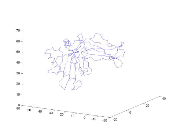
The points represent the shape of a protein. The protein is a one-dimensional chain and each point corresponds to the CA of an amino acid. Connecting them by a curve as embedded in 3D is done by the simple command (in the console of MATLAB):

plot3(x1,y1,z1)

Can you identify secondary structure elements?

Plotting protein structures:

The protein data bank is at www.rcsb.org (Research Collaboratory for Structural Bioinformatics). A gentle introduction to protein structures can be found in:

Carl Branden & John Tooze, “Introduction to Protein Structure”, Garland Publishing NY 1991

PDB files are formatted and include more information that we need or want during this class.

The files open with comments, references and classifications of experimental techniques and structural features. We will be interested in the coordinates. These are lines that start with the keyword ATOM.

Here are typical ATOM entries:

ATOM      1  N   VAL     1      -4.095  14.896  13.982  1.00 17.14      1MBC  88

ATOM      2  CA  VAL     1      -3.483  15.451  15.217  1.00 17.16      1MBC  89

ATOM      3  C   VAL     1      -2.562  14.402  15.817  1.00 15.95      1MBC  90

ATOM      4  O   VAL     1      -2.966  13.230  15.884  1.00 17.17      1MBC  91

ATOM      5  CB  VAL     1      -4.592  15.944  16.184  1.00 18.07      1MBC  92

ATOM      6  CG1 VAL     1      -4.213  17.270  16.885  1.00 17.77      1MBC  93

ATOM      7  CG2 VAL     1      -5.962  16.191  15.584  1.00 19.17      1MBC  94

ATOM      8  N   LEU     2      -1.328  14.772  16.218  1.00 13.50      1MBC  95

ATOM      9  CA  LEU     2      -0.529  13.847  17.019  1.00 11.36      1MBC  96

ATOM     10  C   LEU     2      -1.183  13.755  18.420  1.00  9.99      1MBC  97

ATOM     11  O   LEU     2      -1.582  14.772  18.921  1.00  8.99      1MBC  98

ATOM     12  CB  LEU     2       0.983  14.248  17.119  1.00 10.10      1MBC  99

ATOM     13  CG  LEU     2       1.692  14.001  15.751  1.00  9.73      1MBC 100

ATOM     14  CD1 LEU     2       1.216  14.865  14.716  1.00  8.79      1MBC 101

ATOM     15  CD2 LEU     2       3.147  14.217  16.051  1.00  9.54      1MBC 102

ATOM     16  N   SER     3      -1.114  12.521  18.854  1.00  9.53      1MBC 103

ATOM     17  CA  SER     3      -1.383  12.274  20.256  1.00 10.47      1MBC 104

ATOM     18  C   SER     3      -0.208  12.829  21.090  1.00 10.05      1MBC 105

ATOM     19  O   SER     3       0.833  13.076  20.589  1.00  9.70      1MBC 106

ATOM     20  CB  SER     3      -1.596  10.794  20.556  1.00 10.87      1MBC 107

ATOM     21  OG  SER     3      -0.346  10.023  20.222  1.00 11.48      1MBC 108

ATOM     22  N   GLU     4      -0.513  12.922  22.391  1.00 11.12      1MBC 109

ATOM     23  CA  GLU     4       0.423  13.415  23.392  1.00 11.78      1MBC 110

ATOM     24  C   GLU     4       1.495  12.367  23.459  1.00 11.72      1MBC 111

The second column contains a running index over all the atoms, and the third column contains the atom name. In our first exercise we shall be interested in the CA-s only. The alpha carbons (CA) are at the center of the main chain of the protein. All the different amino acids (named at the fourth column) have the same backbone …N-CA-C… and the CA is at the center of it.

Column 5 lists the index of the amino acid.

Columns 6-8 have the x,y,z coordinate of the corresponding atom.

We shall be interested (at least at the beginning) in a reduced representation of protein structures that will include only CA-s.

Note also that some proteins have more than a single chain. A TERminal line indicates the end of a chain

TER 1070 ARG A 141

In this exercise we use only the first chain in a file.

We need a subroutine that will extract from a protein data bank only the CA of the first chain. The functions crd and word that are given below do just that. They are rather complex and at present we shall not discuss them in details. You may use them as is, or dig into MATLAB help file to understand all of their tricks.

Below is a MATLAB routine that performs this function

function crd = pickCA(pdbFileName)

% Read CA protein data from pdb text file.

fid = fopen(pdbFileName); % Open coordinate file

Eline = fgetl(fid); % Skip till you get to ATOM lines

word = words(Eline); % word-break the line to words separated by space

% ~ is a logical not. Read next line if ~ TER and ~ ATOM

while (and(~strcmp(word{1},'TER'),~strcmp(word{1},'ATOM')))

Fline = fgetl(fid); % The first atom is N

word = words(Fline);

end

% if TER end of chain

if (strcmp(word{1},'TER')) break; end;

Fline = fgetl(fid); % The second atom is CA

word = words(Fline);

%special protein data bank cases are handled below

if or(strcmp(word{5},'R') ,strcmp(word{5},'A'))

x=7; y=8; z=9;

else

x=6; y=7; z=8;

end

i=0;

while (~strcmp(word{1},'TER'))

i = i+1; % The first atom is CA

coords(i,:) = [str2double(word{x}),str2double(word{y}),str2double(word{z})];

while (~strcmp(word{1},'TER'))

Fline = fgetl(fid); % Find the CA of the next amino acid

word = words(Fline);

if strcmp(word{1},'TER') break; end;

if ~strcmp(word{1},'ATOM') break; end;

if strcmp(word{3},'CA') break; end;

end

if or(strcmp(word{1},'TER'),~strcmp(word{1},'ATOM')) break; end;

end

fclose(fid);

crd = coords(1:i,:);

function word = words(string)

% Break a string into whitespace delimited words.

% Produces a cell-array of strings. Individual strings are

% accessed via s{1}, s{2}, and s{3}. Note the curly braces.

s = size(string,2); % Length of input string

blanks = find(isspace(string)); % Find indices of all whitespace

zblanks = [0 blanks]; % 0 counts as whitespace, too

n = size(zblanks,2); % Number of words (includes length 0)

lengths = [blanks s+1] - zblanks - 1; % Lengths of all words

result = cell(1,n); % Reserve space

for i = 1:n % Copy all words (includes length 0)

result{1,i} = string(zblanks(i)+1:zblanks(i)+lengths(i));

end

word = result(lengths > 0); % Remove length 0 words

To read the CA from a protein structure to a MATLAB array do the following:

Connect to www.rcsb.org and extract a protein structure of interest.

Read the file by a call for the above function, in the command window of Matlab.

For example, to extract HUMAN GRANULOCYTE MACROPHAGE COLONY STIMULATING FACTOR with a protein-data-bank (pdb) code – 1gmf:

coor = pickCA('Z:\ron\structures\1gmf.pdb');

coor is a two dimensional array (1:n,1:3). The column is the number of the amino acid and the rows are the x,y,z coordinates

To plot the sequence of CA as a curve in 3D dimension we do:

plot3(coor(:,1),coor(:,2),coor(:,3))

Note that the “:” picks the complete range of the vector and there is no need to know or specify the exact dimension.

The distances between sequential CA in proteins are fixed at approximately 3.8 angstrom, making the connected picture more reasonable.

For many purposes it is useful to set the geometric center of the protein at the origin of the coordinate system (for example, applying a rotation matrix to a system that is not at the origin will have an undesired translational component). The geometric center is defined

In our case the summation is over the coordinates of the CA. A short MATLAB script that set the geometric center of the molecule to zero is below:

n = size(coor,1);

gc = [sum(coor(:,1)) sum(coor(:,2)) sum(coor(:,3))]/n

for i=1:n

coor(i,:) = coor(i,:)-gc;

end

By clicking on the right top bottom it is possible to rotate the protein chain in 3D. It is not that easy to understand properties of the structure from the 3D view. For example, can you identify how many helices are in the structure?

It is useful to have other, less straightforward representations of the structure that are nonetheless simpler to analyze. One interesting representation (in 2D) is the contact matrix. If the distance between a pair of amino acids and is less than seven, the corresponding element in the contact matrix is set to one. Otherwise it is set to zero

A short MATLAB script that prepares and draws a contact map is below:

n = size(coor,1);

counter = 0;

for i=1:n

for j=i+1:n

dist = norm(coor(i,:)-coor(j,:));

if (dist<=7)

counter = counter + 1;

x(counter) = i;

y(counter) = j;

end

plot(x,y,'bd')

We repeat the same exercise for the protein myoglobin (1mbco). Can you suggest a fingerprint for a helix? Beta sheet? Can you identify sharp turns? Explain the off-diagonal elements and what structural features they correspond to.