Notes on integrators of initial value differential equations

We consider differential equations of the type:

-- The Newton’s equation of motion.

Typically a MATLAB function (or other programs) that solves initial value differential equations, takes input of the form

The user provides a function that takes as an input the parameter and returns as an output the value of the derivative of the function -- . The user also provides “initial values”, and the value of the function at some time (for example ). With this information, integrators are able to generate the value of the function at any later time by progressing in small time steps. The simplest integrator of this type is the Euler algorithm:

A process is repeated (e.g. ) to obtain a total desired time of . Note that can be a vector of functions, the same formula will hold for the vector.

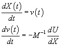
How can we write the Newton’s equations of motions in a form appropriate for the Euler algorithm?

We define an intermediate function (the velocity):

And rewrite the equations of motions as two differential equations of first order

If the motion is along one dimension we can prepare an input for the integrator using the vector definitions:

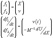
with the initial values: the Euler algorithm can produce the desired trajectory. How accurate is the Euler algorithm? If we are using a Taylor expansion of -- , it is clear that that the local accuracy of the Euler algorithm is . It is quite straightforward to improve the local accuracy (as we will see shortly), however, even more important (and more subtle) is the requirement of global accuracy. It is possible that accurate local solution will have errors that accumulate and after a large number of steps the global error will huge. On the other hand, an algorithm that is not doing great locally, may have errors that do not aggregate, resulting in a sound approximation even after a large number of steps.

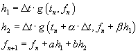
Improvement of local errors is nevertheless useful in a number of cases and we shall look into a class of algorithms that make it possible (Runge Kutta Methods). These improvements however, come at a cost. The cost is usually measured in the number of function (or derivative) evaluations.

The Euler method is using one function evaluation and is accurate to the first order. The Runge Kutta methods can be tuned to the desired accuracy by doing more function evaluations. If highly accurate results are desired the Runge Kutta techniques are the method of choice, with sufficiently small time step we can make the solution (locally) very accurate. Here is an example of the design of a Runge Kutta method of a second order accuracy. Define

We have four unknown parameters: that we wish to determine so that the local error will be of the order . This is done below

First we write a straightforward Taylor expansion of . Then we shall use the above alternative derivation of the function at the next time () and compare the two terms

First derivation of the future value of the function:

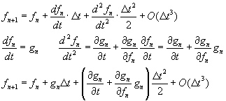
Where the third expression is obtained after substituting the derivative expressions (second line) in the first equation.

Second derivation of the future value of the function:

All the above equations are computed at step or time . We still need to compute , in order to arrive at the alternative derivation. By expanding to the first order in we obtain:

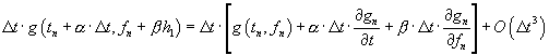
Now we are ready to write our estimate for the function at the next time using the four parameters

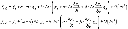
But this function must be equal to the regular Taylor expansion:

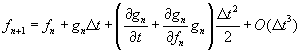
We therefore have

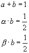
There are three equations and four unknowns. So there is infinite number of solutions. A choice is: .

The algorithms is written as: