Can we prove that a program works for all possible inputs. In principle, yes. In practice, this approach is too time-consuming to be applied to large programs. However, it is useful to look at how proofs of correctness can be constructed:
What is a proof? A completely convincing argument that something is true. For an argument to be completely convincing, it should be made up of small steps, each of which is obviously true. In fact, each step should be so simple and obvious that we could build a computer program to check the proof. We need two ingredients make this possible:
A logic accomplishes these two goals.
The strategy for proving programs correct will be to convert programs and their specifications into a purely logical statement that is either true or false. If the statement true, then the program is correct. To really make sure our proofs are convincing, we need a clear understanding of what a proof is.
Curiously, mathematicians did not really study the proofs that they were constructing until the 20th century. Once they did, they discovered that logic itself was a deep topic with many implications for the rest of mathematics.
We start with propositional logic, which is a logic built up from simple symbols representing propositions about some world. For our example, we will use the letters A, B, C, ... as propositional symbols. For example, these symbols might stand for various propositions:
It is not the job of propositional logic to assign meanings to these symbols. However, we use statements to the meanings of D and E to talk about the correctness of programs.
We define a grammar for propositions built up from these symbols. We use the letters P, Q, R to represent propositions (or formulas):
P,Q,R ::= ⊤                    (* true *)
        | ⊥                    (* false *)
        | A, B, C              (* propositional symbols *)
        | ¬P                   (* sugar for P⇒⊥ *)
        | P∧Q                  (* "P and Q" (conjunction) *)
        | P∨Q                  (* "P or Q" (disjunction) *)
        | P⇒Q                  (* "P implies Q" (implication) *)
Note: On some browsers in some fonts the symbol for and (in the fonts used here: ∧, ∧) is rendered incorrectly as a small circle. It should look like an upside-down V.
The precedence of these forms decreases as we go down the list, so P∧Q⇒R is the same as (P∧Q)⇒R. One thing to watch out for is that ⇒ is right-associative (like →), so P⇒Q⇒R is the same as P⇒(Q⇒R). We will introduce parentheses as needed for clarity. We will use the notation for logical negation, but it is really just syntactic sugar for the implication P⇒⊥.
This grammar defines the language of propositions. With suitable propositional symbols, we can express various interesting statements, for example:
In fact, all three of these propositions are logically equivalent, which we can determine without knowing about what finals and attendance mean.
In order to say whether a proposition is true or not, we need to understand what it means. The truth of a proposition sometimes depends on the state of the "world". For example, proposition D above is true in a world where x=0 and y=10, but not in a world in which x=y=0. To understand the meaning of a proposition P, we need to know whether for each world, it is true. To do this, we only need to know whether P is true for each possible combination of truth or falsity of the propositional symbols A,B,C,... within it. . For example, consider the proposition A∧B. This is true when both A and B are true, but otherwise false. We can draw a truth table that describes all four possible worlds compactly:
| ∧ | false | true | A |
|---|---|---|---|
| false | false | false | |
| true | false | true | |
| B |
This kind of table can also be used to describe the action of an operator like ∧ for a conjunction over general propositions P∧Q rather than over simple propositional symbols A and B. Here is a truth table for disjunction. Notice that in the case where both P and Q are true, we consider P∨Q to be true. The connective ∨ is inclusive rather than exclusive.
| ∨ | false | true | P |
|---|---|---|---|
| false | false | true | |
| true | true | true | |
| Q |
We can also create a truth table for negation ¬P:
| ¬ | false | true | P | |
|---|---|---|---|---|
| false | true | false |
Implication P⇒Q is tricky. The implication seems true if P is true and Q is true, and if P is false and Q is false. And the implication is clearly false if P is true and Q is false:
| ⇒ | false | true | P |
|---|---|---|---|
| false | true | false | |
| true | ? | true | |
| Q |
What about the case in which P is false and Q is true? In a sense we have no evidence about the implication as long as P is false. Logicians consider that in this case the assertion P⇒Q is true. Indeed, the proposition P⇒Q is considered vacuously true in the case where P is false, yielding this truth table:
| ⇒ | false | true | P |
|---|---|---|---|
| false | true | false | |
| true | true | true | |
| Q |
We can use truth tables like these to evaluate the truth of any propositions we want. For example, the truth table for (A⇒B)∧(B⇒A) is true in the places where both implications would be:
| ⇔ | false | true | A |
|---|---|---|---|
| false | true | false | |
| true | false | true | |
| B |
In fact, this means that A and B are logically equivalent, which we write as A iff B or A⇔B. If P⇔Q, then we can replace P with Q wherever it appears in a proposition, and vice versa, without changing the meaning of the proposition. This is very handy.
Another interesting case is the proposition (A∧B)⇒B. The truth table looks like this:
| (A∧B)⇒B | false | true | A |
|---|---|---|---|
| false | true | true | |
| true | true | true | |
| B |
In other words, the proposition (A∧B)⇒B is true regardless of what A and B stand for. In fact, it will be true if A and B are replaced with any propositions P and Q. We call such a proposition a tautology.
There are a number of useful tautologies, including the following:
| Associativity | (P∧Q)∧R ⇔ (P∧Q)∧R | (P∨Q)∨R ⇔ (P∨Q)∨R | |
| Symmetry | (P∧Q) ⇔ (Q∧P) | (P∨Q) ⇔ (Q∨P) | |
| Distributivity | P∧(Q∨R) ⇔ (P∧Q)∨(P∧R) | P∨(Q∧R) ⇔ (P∨Q)∧(P∨R) | |
| Idempotency | P∧P ⇔ P | P∨P ⇔ P | |
| DeMorgan's laws | ¬(P∧Q) ⇔ ¬P∨¬Q | ¬(P∨Q) ⇔ ¬P∧¬Q | |
| Negation | P ⇔ ¬¬P | P⇒⊥ ⇔ ¬P | P⇒Q ⇔ ¬P∨Q |
These can all be derived from the rules we will see shortly, but they are useful to know.
Notice that we can use DeMorgan's laws to turn ∧ into ∨, and use the equivalence P⇒Q ⇔ ¬P∨Q to turn ∨ into ⇒, and the equivalence P⇒⊥ ⇔ ¬P to get rid of negation. So we can express any proposition using just implication ⇒ and the false symbol ⊥!
To prove whether propositions are true without testing every possible world, we need a system for deduction. We can construct proofs of a proposition by using inference rules to derive the desired proposition starting from axioms.
The most famous inference rule is known as modus ponens. Intuitively, this says that if we know P is true, and we know P⇒Q, then we can conclude Q:
| (modus ponens) | ||||
The propositions above the line are the premises; the proposition below the line is the conclusion. Both the premises and the conclusion may contain metavariables (in this case, P and Q), representing arbitrary propositions. When a inference rule is used as part of a proof, the metavariables are replaced in a consistent way with the appropriate kind of object (in this case, propositions).
Most rules come in one of two flavors: introduction or elimination rules. Introduction rules introduce the use of a logical operator, and elimination rules eliminate it. For example, introduction and elimination rules for ∧ can be written as follows:
| (∧I) | ||||
| (∧E1) |
| (∧E2) |
Together, a set of inference rules make up a proof system that determines what can be proved. There is still something important missing from our proof system; how can we prove an implication P⇒Q? Intuitively, the way this is proved is by assuming that P is true, and with that assumption, showing that Q is true too. To keep track of assumptions, we introduce a new notation, P⊢Q, which means “if we assume P is true, we can prove Q.” The symbol ⊢ is called a turnstile. The statement ⊢Q means Q can be proved without any assumptions. In general, we may need to have several outstanding assumptions. We write Γ to represent a set of assumptions, and our proof rules are expressed in terms of sequents with the form Γ⊢P. For example, we can always prove P⊢P, or in general, Γ,P⊢P for any set of assumptions Γ and proposition P. This is the general rule for introducing a new assumption:
| (assumption) |
Because it has no premises, this rule is an axiom: something that can start a proof.
It is also okay to add new assumptions through the weakening rule:
| (weakening) |
In other words, if you can prove P using assumptions Γ, you can certainly prove P using Γ plus an added assumption Q. The key to the proof system is that assumptions can only be removed by using the introduction rule for ⇒.
We can introduce an implication P⇒Q by showing P⊢Q, and eliminate an ⇒ with modus ponens (extended to keep track of assumptions):
| (⇒I) |
| (⇒E, modus ponens) | ||||||
The rules we have already seen for conjunction and implication can be extended to keep track of assumptions, too:
| (∧I) |
| (∧E1) |
| (∧E2) | ||||||||
The introduction and elimination rules for disjunction are as follows:
| (∨ intro 1) |
| (∨ intro 2) | |||||
| (∨ elim) | |||||||
Finally, some rules relating to negation:
| (special case of ⇒I) |
| (RAA, reductio ad absurdum) | ||||
| (false proves everything) |
Reductio ad absurdum is an interesting rule. It says that if the negation of a proposition can be used to prove falsity, the proposition must be true. This rule is present in classical logic but not in constructive logics, in which things cannot be proved true simply by showing the falsity of their negations. In constructive logics, the the law of the excluded middle, P∨¬P, does not hold. However, we will use this rule.
A proof of proposition P in natural deduction starts from axioms and derives the judgement ⊢P; that is, it proves P under no assumptions. Every step in the proof is an instance of an inference rule with metavariables substituted consistently with expressions of the appropriate syntactic class.
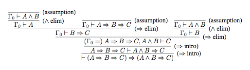
For example, here is a proof of the proposition (A⇒B⇒C) ⇒ (A∧B⇒C). For brevity, Γ₀ is used as an abbreviation for the assumptions (A⇒B⇒C), A∧B.
The final step in the proof is to derive ⊢(A⇒B⇒C) ⇒ (A∧B⇒C) from (A⇒B⇒C) ⊢ (A∧B⇒C), which is done using the rule (⇒ intro). To see how this rule generates the proof step, substitute for the metavariables P, Q, and Γ as follows: P = (A⇒B⇒C), Q = (A∧B⇒C), Γ = Ø. The immediately previous step uses the same rule, but with a different substitution: P = A∧B, Q = C, Γ = (A⇒B⇒C).
This shows that a proof of proposition P is a tree generated by inference rules. The leaves of the tree are axioms and the root is P. If we represent each proposition in this proof as a node in a tree, we get the following:

Writing out proofs at this level of detail can be a bit tedious. But notice that checking the proof is completely mechanical, requiring no intelligence or insight whatever. Therefore it is a very strong argument that the thing proved is in fact true.
We can also make writing proofs like this less tedious by adding more rules that provide reasoning shortcuts. These rules are sound (they only prove true things), if there is a way to convert a proof using them into a proof using the original rules. Such added rules are called admissible.
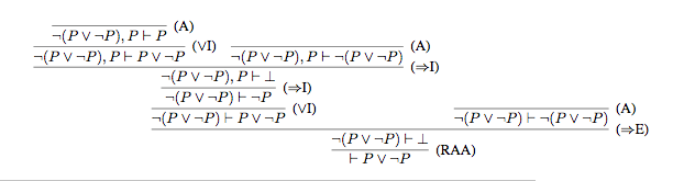
For any proposition P, we can use our logic to prove the law of the excluded middle: P∨¬P. Abbreviating "intro" as I, "elim" as E, and "assumption" as A, we have this proof tree (notice that we did need to use the non-constructive reductio ad absurdum rule to prove this):
In propositional logic, the statements we are proving are completely abstract. To be able to prove programs correct, we need a logic that can talk about the things that programs compute on: integers, strings, tuples, datatype constructors, and functions. We'll enrich propositional logic with the ability to talk about these things, obtaining a version of predicate logic.
The syntax extends propositional logic with a few new expressions, shown in blue:
P,Q,R ::= ⊤                    (* true *)
        | ⊥                    (* false *)
        | A, B, C              (* propositional symbols *)
        | ¬P                   (* sugar for P⇒⊥ *)
        | P∧Q                  (* "P and Q" (conjunction) *)
        | P∨Q                  (* "P or Q" (disjunction) *)
        | P⇒Q                  (* "P implies Q" (implication) *)
	| ∀x.P                 (* P is true for all x. P can mention x*)
	| ∃x.P                 (* There exists some x such that P is true *)
	| e1 = e2               (* e1 is equal to e2 *)
	| p(e)                 (* The predicate named p is true for e *)

e ::=     v                    (* integers, tuples, other SML values *)
        | x                    (* The name of a value, may be bound
	                           by ∀ or ∃ *)
	| f(e)                 (* Result of applying function
	                          named f to e *)
The formula ∀x.P means that the formula P is true for any choice of x. This is called universal quantification, and ∀ is the universal quantifier. The formula ∃x.P denotes existential quantification. It means that the formula P is true for some choice of x, though there may be more than one such x. Existential and universal quantifiers can be turned into each other using negation. The formula ∃x.P is equivalent to ¬∀x.¬P, because if there exists some x that makes P true, then clearly ¬P is not true for all x. Similarly, the formula ∀x.P is equivalent to ¬∃x.¬P. These equivalences are generalizations of DeMorgan's to existential and universal quantifiers.
We will assume that we can tell from the name of x what type of thing it is. What if we want to restrict to talking about some subset? For universal quantifiers, the trick is to use an a For example, if we want to say that all numbers greater than one are also greater than zero, we write ∀x.x>1⇒x>0. This works because the quantified formula is vacuously true for the numbers not greater than 1. If we want to limit the range in an existential, we use conjunction. For example, to say that there exists a number greater than zero that is greater than one, we write ∃x.x>0∧x>1.
Using quantifiers, we can express some interesting statements. For example, we can express the idea that a number n is prime (note m and k are integers) in various logically equivalent ways:
| prime(n) | ⇔ | ∀m.1<m∧m<n⇒¬∃k.k*m = n |
| ⇔ | ¬∃m.1<m∧m<n∧∃k.k*m = n (DeMorgan's laws) | |
| ⇔ | ¬∃m.∃k.1<m∧m<n∧k*m = n |
This example shows one fine point of syntax: when reading quantifiers ∀x.P, the formula P extends as far to the right as possible. So (∀m.1<m∧m<n⇒¬∃k.k*m = n) is read as (∀m.1<m∧m<n⇒(¬∃k.k*m = n)) rather than as (∀m.1<m∧m<n)⇒(¬∃k.k*m = n). This is the same as for other perhaps more familiar binding constructs, such as summation ∑ and integrals ∫.
Introduction and elimination rules can be defined for universal and existential quantifiers. The rules for universals are as follows:
| (∀I) |
| (∀E) | ||||||
We use the notation FV(Γ) to indicate the free variables of the assumptions Γ, that is, the variables that occur in an unbound occurrence. The requirement in (∀I) that x∈FV(Γ) prevents us from doing unsound generalizations like the following:
| x>0 ⊢ x>1 |
| x>0 ⊢ ∀x. x>1 |
The rule (∀E) specializes the formula P to a particular value of x. We require implicitly that e be of the right type to be substituted for x. Since P holds for all x, it should hold for any given choice of x, that is, e.
The rules for existentials are as follows:
| (∃I) |
| (∃E) | ||||||||
The rule (∃I) derives ∃x.P because a witness to the existential has been produced. The idea behind rule (∃E) is that if something (Q) can be shown that doesn't mention on the witness (x), then it is true without the existential: ∃x.Q is the same as Q if Q doesn't mention x.
The predicate logic allows the use of arbitary predicates p. Equality is a predicate that applies to two arguments; we can read e1=e2 alternatively as a predicate =(e1,e2). We support reasoning about predicates by adding rules (esp. axioms) Equality is special because when two things are equal, one can be substituted for the other in any context.
The following three rules capture that equality is an equivalence relation: it is reflexive, symmetric, and transitive.
| (refl) |
| (symm) |
| (trans) | ||||||||
Beyond being an equivalence relation, equality preserves meaning under substitution. If two things are equal, substituting one for the other in equal terms results in equal terms:
| ||||
However, this rule can be generalized. First, it applies to arbitrary formulas, not just to equality formulas e1 = e2. Second, it is not necessary to replace all occurrences of x. The truth of the formula is unchanged if only some occurrences are changed. We write the rule with a variable z to indicate where the occurrences of x to be changed are located. Third, it applies to arbitrary equalities, not just equalities involving a variable x:
| ||||
The same idea can be applied at the propositional level as well. If we can prove that two formulas are equivalent, they can be substituted for one another within any other formula:
| ||||
Also we don't in principle need this rule to proofs, it can be very handy for logical reasoning, especially with a large “library” of logical equivalences to draw upon.
For reasoning about specific kinds of values, we need axioms that describe how those values behave. For example, the following axioms partly describe the integers and can be used to prove many facts about integers. In fact, they define a more general structure, a commutative ring, so anything proved with them holds for any commutative ring.
| ⊢ ∀x.∀y.x+y=y+x | (commutativity of +) |
| ⊢ ∀x.∀y.∀z.(x+y)+z = x+(y+z) | (associativity of +) |
| ⊢ ∀x.∀y.∀z.(x*y)*z = x*(y*z) | (associativity of *) |
| ⊢ ∀x.∀y.∀z.x*(y+z) = x*y+x*z | (+ distributes over *) |
| ⊢ ∀x.x + 0 = x | (additive identity) |
| ⊢ ∀x.x + (-x) = 0 | (additive inverse) |
| ⊢ ∀x.x*1=x ∧ 1*x=x | (multiplicative identity) |
| ⊢ ¬0=1 | |
| ⊢ ∀x.∀y.x*y=y*x | (commutativity of *) |
These rules use a number of functions: +, *, -, 0, and 1 (we can think of 0 and 1 as functions that take zero arguments). These symbols are represented by the metavariable f in the grammar earlier.
Proving facts about arithmetic can be tedious. For our purposes, we will write proofs that do reasonable algebraic manipulations as a single step, e.g.
| (algebra) | |||
This step can be done explicitly using the rules and axioms above, but it takes several steps.
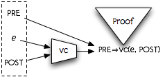
Our goal is to prove programs correct. Our strategy is to turn a program into a logical formula whose truth corresponds to the correctness of the program. We need not only the code of the program, but also a specification of what the program is supposed to do. This specification will be expressed as two logic formulas: a precondition describing what can be assumed to be before the program executes, and a postcondition describing what must be true after the program executes. Given this triple of (precondition, program, postcondition), we want to produce a logical formula called the verification condition, which implies that that starting with the precondition true and executing the program, the postcondition will be true. Then we can show that the program is correct by producing a proof that the formula is true.
To produce this formula, we will use the program code and the desired postcondition to generate a precondition that ensures the postcondition. If the actual precondition implies this precondition, the program must be correct. We define a function vc(e, r, P) which produces a logical formula with the following meaning (“vc” for verification condition):
vc(e, r, P) is a formula Q such that if e is evaluated when the precondition Q is true, and its result is placed in the variable r, the postcondition P will be true.
Given this definition, given code e, precondition PRE, and postcondition POST, the actual verification condition for the program is:
We can depict this approach to program verification as follows:
For example, consider the very simple program e = y+1. If we give the name r to the result of evaluating e, and want to ensure the postcondition r>10, what is the weakest precondition that will ensure this? Clearly, if y+1>10 (or equivalently, y>9). Therefore, we'd like to define that vc(y+1, r, r>10) is (y+1 > 10). Then, if for example we have a precondition that y ≥ 15, we can reduce the correctness of the program to the truth of the formula y ≥15 ⇒ y+1 > 10.
Let us use the metavariable “a” to represent an SML expression that can
also appear as an expression in the logic. Expressions of this form can
use functions and predicates that are useful for writing specifications;
we will also let them use SML constructors such as tuple constructors and
datatype constructors. For example, the expression y+1
is such an expression.
The vc rule for an expression a is very simple:
P{a/r}
In other words, we substitute the expression a for the variable r. In fact, we already used this rule for the previous example, where we decided the weakest precondition is (r>10){y+1/r} = (y+1>10).
Next, consider the expression
let x = e1 in e2 end. The result of
this expression is whatever e2 evaluates to, so intuitively
we need to satisfy vc(e2, r, P). However, e2 may
depend on x, so the real precondition is that e1 should evaluate
to something named x such that the evaluation of e2 satisfies P:
let val x = e1 in e2 end, r, P) =
vc(e1, x, vc(e2, r, P))
Example:
vc(let val y=z+1 in y*y end, r, r>0)
| |
| = | vc(z+1, y, vc(y*y, r, r>0))
|
| = | vc(z+1, y, y*y>0)
|
| = | (z+1)*(z+1)>0 |
| ⇔ | z≠−1 |
For an if expression, there are two possible execution paths,
and the postcondition must be satisfied in both paths. Therefore, we use
a conjunction over preconditions for these two cases:
if a then e1 else e2, r, P) =(a ⇒ vc(e1, r, P)) ∧ (¬a ⇒ vc(e2, r, P))
Example:
vc(if y>z then y else z, r, r>0)
| ||
| = | (y>z ⇒ vc(y, r, r>0))
∧ (y≤z ⇒ vc(z, r, r>0))
| |
| = | (y>z ⇒ y>0) ∧ (y≤z ⇒ z>0) | |
| ⇔ | (y≤z ∨ y>0) ∧ (y>z ∨ z>0) | (De Morgan) |
| ⇐ | y>0 ∨ z>0 |
Notice that we assumed that the condition was a simple expression a
that could appear in the logic. We can always desugar more complex if's and
determine the vc accordingly:
vc(if e0 then e1 else e2, r, P)
| ||
| = | vc(let val x=e0 in if x then e1 else e2 end, r, P) | (where x is a fresh variable) |
| = | vc(e0, x, vc(if x then e1 else e2, r, P))
| |
| = | vc(e0, x, x⇒vc(e1, r, P)∧(¬x)⇒vc(e2, r, P))
|
Therefore subsequent rules will often assume that subexpressions have simple form.
One other important expression is case, which is like
if in that there are multiple alternative expressions to evaluate.
We write two rules, one for a case with multiple arms, and another for a
case with a single arm. In both rules we assume there there is
a set of variables xi that are bound in the pattern p
case a of p => e | ... , r, P) =case a of ..., r, P))
case a of p => e, r, P) =To reason about datatypes, we need some axioms. Suppose we have a datatype declaration:
datatype t = X1 of t1 | ... | Xn of tn
Then we have axioms saying that any value x of type t matches
exactly one of these constructors, with corresponding argument yi
of type ti:
And all of these constructors are disjoint: for every i and j, 1≤i≤n, 1≤j≤n,
We verify functions in a modular style, using function specifications. For each function, we prove that it satisfies its spec. We then assume that the function satisfies its specification when reasoning about code that uses the function. Let's assume that we have specifications written in the following style:
(* Requires: Q
 * Returns: r = f(x) where P
 *)
fun f(x) = e
The Requires clauses is the precondition, and talks about the formal parameter x. In general the function may mention some other formal parameter name; we will use the notation arg(f) to represent the declared formal parameter. The Returns clause gives the postcondition P. We assume that it expresses conditions on the result of the function by naming it as some variable result(f), which is r in this case. We write pre(f) to refer to the precondition Q, and post(f) to refer to the postcondition P.
Then we can capture the correctness of the implementation of f in the following formula:
When a function f is applied to an argument a, we assume that f is implemented correctly. In other worse, the verification precondition should be that the precondition of the function is satisfied, and that the postcondition of the function implies the desired postcondition. However, the uses of arg(f) and result(f) in the precondition and postcondition need to be replaced by the actual argument a and the desired result variable r:
pre(f){a/arg(f)} ∧ (post(f){a/arg(f), r/result(f)} ⇒ P)
Let's use this to prove that a function that computes the maximum of two numbers is correct:
(* Requires: true
 * Returns: r where (r=x ∨ r=y) ∧ r≥x ∧ r≥y
 *)
fun max(x:int, y:int) =
   if x > y then x else y
We want to show pre(max) ⇒ vc(if x > y then x else y, result(max), post(max)), which is:
| pre(max) ⇒ vc(if x > y then x else y, result(max), post(max)) | ||
| = | true ⇒ vc(if x > y then x else y, result(max), post(max)) | |
| = | vc(if x > y then x else y, result(max), post(max)) | (Note: true⇒P ⇔ P) |
| = | (x>y ⇒ vc(x, r, post(max))) ∧ (x≤y ⇒ vc(y, r, post(max))) | |
| = | (x>y ⇒ post(max){x/r}) ∧ (x≤y ⇒ post(max){y/r}) | |
| = | (x>y ⇒ (x=x ∨ x=y) ∧ x≥x ∧ x≥y) ∧ (x≤y ⇒ (y=x ∨ y=y) ∧ y≥x ∧ y≥y) | |
| ⇔ | (x>y ⇒ x≥y) ∧ (x≤y ⇒ y≥x) | |
| ⇔ | (T∧T) | |
| ⇔ | T |
Therefore the implementation is correct.
Now, suppose we want to show that the following function that finds the maximum element in a list is correct:
(* Requires: l ≠ nil
 * Returns: the maximum element of the list. That is, r where
            r∈l ∧ ∀x. x∈l ⇒ r≥x
 *)
fun lmax(l) =
  case l of
    [y] => y
  | h::t => let val m = lmax(t) in
	      max(m,h)
	    end
We need to prove l≠nil ⇒ vc(case l of ..., r, post(lmax)). We also need to define the predicate ∈ for membership in a list for this spec to make sense: x∈l ⇔ ∃h.∃t.l=h::t ∧ (h=x ∨ x∈t). (Technically, this predicate is defined recursively, by induction on the length of the list l.) Expanding out the definition of vc for the function body and performing some logical simplifications, we have:
| l≠nil ⇒ vc(case l of ..., r, post(lmax)) | |
| = |
l≠nil ⇒ (l = x::nil ⇒ vc(y, r, post(lmax))) ∧ (¬∃y. l=y::nil) ⇒ vc(case l of h::t => let ..., r, post(lmax)) |
| = |
l≠nil ⇒ (l = y::nil ⇒ post(lmax){y/r})) ∧ (¬∃y. l=y::nil) ⇒ vc(case l of h::t => let ..., r, post(lmax)) |
| = | l≠nil ⇒ (l = y::nil ⇒ y∈l ∧ ∀x. x∈l ⇒ y≥x) ∧ (¬∃y. l=y::nil) ⇒ vc(case l of h::t => let ..., r, post(lmax)) |
To prove this, we can separately prove the conjuncts inside
the consequent, starting with the first (blue), which captures the correctness
of the first arm of the case. Here are the first steps of
that proof:
| l≠nil, l = y::nil ⊢ y∈l |
| ||
| l≠nil, l = y::nil ⊢ y∈l ∧ ∀x. x∈l ⇒ y≥x |
| l≠nil ⇒ l = y::nil ⇒ (y∈l ∧ ∀x. x∈l ⇒ y≥x) |
Now let's look at the second conjunct, corresponding to the second arm:
| l≠nil ⇒ ¬∃y. l=y::nil ⇒ vc(case l of h::t => let ..., r, post(lmax)) | |
| = | l≠nil ⇒ ¬∃y. l=y::nil ⇒ vc(case l of h::t => let ..., r, post(lmax)) |
| = | l≠nil ⇒ ¬∃y. l=y::nil ⇒ ((l = h::t ⇒ vc(let ..., r, post(lmax)))∧∃h.∃t.l=h::t) |
| = | (l≠nil ∧ ¬∃y. l=y::nil) ⇒ ((l=h::t ⇒ vc(let val m = lmax(t) in max(m,h) end, r, post(lmax)))∧∃h.∃t.l=h::t) |
| = | (l≠nil ∧ ¬∃y. l=y::nil) ⇒ ((l=h::t ⇒ vc(lmax(t), m, vc(max(m,h), r, post(lmax))))∧∃h.∃t.l=h::t) |
Now we can use the specs for max and lmax to simplify further:
| vc(lmax(t), m, vc(max(m,h), r, post(lmax))) | |
| = | pre(lmax){t/l} ∧ (post(lmax){t/l, m/r} ⇒ vc(max(m,h), r, post(lmax))) |
| = | t≠nil ∧ ((m∈t∧∀x.x∈t⇒m≥x) ⇒ vc(max(m,h), r, post(lmax))) |
| = | t≠nil ∧ ((m∈t∧∀x.x∈t⇒m≥x) ⇒ (pre(max){m/x,h/y} ∧ post(max){m/x,h/y} ⇒ post(lmax))) |
| = | t≠nil ∧ ((m∈t∧∀x.x∈t⇒m≥x) ⇒ (T ∧ ((r=m ∨ r=h) ∧ r≥m ∧ r≥h) ⇒ post(lmax))) |
| = | t≠nil ∧ ((m∈t∧∀x.x∈t⇒m≥x) ⇒ (((r=m ∨ r=h) ∧ r≥m ∧ r≥h) ⇒ r∈l ∧ ∀x. x∈l ⇒ r≥x)) |
Putting this back into the second conjunct, we have:
This can be proved using the datatype axioms for lists.