So far we've been programming as though all pointers between boxes are equally expensive to follow. This turns out not to be even approximately true. Our simple model of how the computer memory works was that the processor generates requests to the memory that include a memory address. The memory looks up the appropriate data and sends it back to the processor. Computers used to work this way, but these days processors are so much faster than memory that something else is needed. A typical computer memory these days takes about 60ns to deliver requested data. This sounds pretty fast, but you have to keep in mind that a 2GHz processor is doing a new instruction every 0.5ns. Thus, the computer will have to wait for about 100 cycles every time the memory is needed to deliver data.
This problem is solved by sticking smaller, faster memory chips in between the processor and the main memory. These chips are called a cache : a cache keeps track of the contents of memory locations that were recently requested by the processor. Because the cache is much smaller than main memory (hundreds of kilobytes instead of tens or hundreds of megabytes), it can be made to deliver requests much faster than main memory: in tens of cycles rather than hundreds. In fact, one level of cache isn't enough. Typically there are two or three levels of cache, each smaller and faster than the next one out. The primary cache is the fastest cache, usually right on the processor chip and able to serve memory requests in one or two cycles. The secondary cache is larger and slower. Tertiary caches, if used, are usually off-chip.
For example, the next-generation Intel processor (Itanium2) has three levels of cache right on the chip, with increasing response times (measured in processor cycles) and increasing cache size. The result is that almost all memory requests can be satisfied without going to main memory.
Having caches only helps if when the processor needs to get some data, it is already in the cache. Thus, the first time the processor access the memory, it must wait for the data to arrive. On subsequent reads from the same location, there is a good chance that the cache will be able to serve the memory request without involving main memory. Of course, since the cache is much smaller than the main memory, it can't store all of main memory. The cache is constantly throwing out information about memory locations in order to make space for new data. The processor only gets speedup from the cache if the data fetched from memory is still in the cache when it is needed again. When the cache has the data that is needed by the processor, it is called a cache hit. If not, it is a cache miss. The ratio of the number of hits to misses is called the cache hit ratio. Because memory is so much slower than the processor, the cache hit ratio is critical to overall performance.
Caches improve performance when memory accesses exhibit: reads from memory tends to request the same locations repeatedly, or at least memory locations near previous requests. A tendency to revisit the same or nearby locations is known as locality. Computations that exhibit locality will have a relatively high cache hit ratio. Note that caches actually store chunks of memory rather than individual words of memory. So a series of memory reads to nearby memory locations are likely to mostly hit in the cache. When there is a cache miss, a whole sequence of memory words is requested from main memory at once, because it is cheaper to read memory that way. The cache records cached memory locations in units of cache lines whose size depends on the size of the cache (typically 4-32 words).
How does this affect us as programmers? We would like to write code that has good locality to get the best performance. This has implications for many of the data structures we have looked at. For example, we talked about how to implement hash tables using linked lists to represent the buckets. Linked lists involve chasing a lot of pointers, which means they have poor locality. A given linked list node probably doesn't even fill up one cache line. When the node is accessed, the whole cache line is fetched from main memory, yet it is mostly not used.
For best performance, you should figure out how many elements can be fit sequentially into a single cache line. The representation of a bucket set is then a linked list where each node in the linked list contains several elements (and a chaining pointer) and takes up an entire cache line. Thus, we go from a linked list that looks like the one on top to the one on the bottom:

Doing this kind of performance optimization can be tricky in a language like SML where the language is working hard to hide these kind of low-level representation choices from you. In languages like C, C++, or Modula-3, you have the ability to control memory layout somewhat better. A rule of thumb, however, is that SML records and tuples are stored contiguously in memory. So this kind of memory layout can be implemented in SML, e.g.:
datatype bucket = Empty | Bucket of elem * bucket (* poor locality *)
datatype big_bucket =
  BigEmpty
| Bucket of {e1: elem, e2: elem, e3: elem, next: big_bucket} (* better locality *)
The same idea can be applied to trees. Binary trees are not good for locality because a given node of the binary tree probably occupies only a fraction of a cache line. B-trees are a way to get better locality. As in the hash table trick above, we store several elements in a single node -- as many as will fit in a cache line.
B-trees were originally invented for storing data structures on disk, where locality is even more crucial than with memory. Accessing a disk location takes about 5ms = 5,000,000ns. Therefore if you are storing a tree on disk you want to make sure that a given disk read is as effective as possible. B-trees, with their high branching factor, ensure that few disk reads are needed to navigate to the place where data is stored. B-trees are also useful for in-memory data structures because these days main memory is almost as slow relative to the processor as disk drives were when B-trees were introduced!
A B-tree of order m is a search tree where each nonleaf node has up to m children. The actual elements of the collection are stored in the leaves of the tree. The data structure satisfies several invariants:
For example, the following is an order-5 B-tree (m=5) where the leaves have enough space to store up to 3 data records:

Because the height of the tree is uniformly the same and every node is at least half full, we are guaranteed that the asymptotic performance is O(lg n) where n is the size of the collection. The real win is in the constant factors, of course. We can choose m so that the pointers to the m children plus the m−1 elements fill out a cache line at the highest level of the memory hierarchy where we can expect to get cache hits. For example, if we are accessing a large disk database then our "cache lines" are memory blocks of the size that is read from disk.
Lookup in a B-tree is straightforward. Given a node to start from, we use a simple linear or binary search to find whether the desired element is in the node, or if not, which child pointer to follow from the current node.
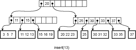
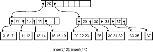
Insertion and deletion from a B-tree are more complicated; in fact, they are notoriously difficult to implement correctly. For insertion, we first find the appropriate leaf node into which the inserted element falls (assuming it is not already in the tree). If there is already room in the node, the new element can be inserted simply. Otherwise the current leaf is already full and must be split into two leaves, one of which acquires the new element. The parent is then updated to contain a new key and child pointer. If the parent is already full, the process ripples upwards, eventually possibly reaching the root. If the root is split into two, then a new root is created with just two children, increasing the height of the tree by one.
For example, here is the effect of a series of insertions. The first insertion merely affects a leaf. The second insertion overflows the leaf and adds a key to an internal node. The third insertion propagates all the way to the root.


Deletion works in the opposite way: the element is removed from the leaf. If the leaf becomes empty, a key is removed from the parent node. If that breaks invariant 3, the keys of the parent node and its immediate right (or left) sibling are reapportioned among them so that invariant 3 is satisfied. If this is not possible, the parent node can be combined with that sibling, removing a key another level up in the tree and possible causing a ripple all the way to the root. If the root has just two children, and they are combined, then the root is deleted and the new combined node becomes the root of the tree, reducing the height of the tree by one.
Further reading: Aho, Hopcroft, and Ullman, Data Structures and Algorithms, Chapter 11.