Problem Set 5: Parallel Sequences and N-Body Simulation
Due April 12, 2012
Important notes:
- Partners: You may work on this problem set with a
partner.
- Compile errors: All programs you submit must
compile. Programs that do not compile will receive a
zero. If you are having trouble getting your assignment to
compile, please visit consulting hours. If you run out of time, it
is better to comment out the parts that do not compile and hand in a
file that compiles than hand in a more complete file that does not
compile.
- Function names: We will use an automatic grading
script, so it is crucial that you name your
functions and order their arguments according to the problem set
instructions, and that you place the functions in the correct files.
Otherwise you may not receive credit for a function properly
written.
- Style: Pay attention to style. Refer to the CS 3110
style guide and lecture notes. Ugly code that is functionally
correct may still lose points. Take the extra time to think through
each problem and find an elegant solution before coding it up.
- Versions: Please double-check that the files you submit
to CMS are the correct versions.
Changelog
- The flatten function does not require a parallel
implementation. You may use any correct, functional implementation without
worrying about the work and span complexity.
Part 1: Source Control (3 points)
For this assignment, you must use a version control system such as Git
or SVN and submit the log file that describes the activity on your
repository. We will provide you with an SVN repository hosted by
CSUG. Note: if you use Git, you should not host your code on a public
repository such as GitHub, as making your code available to others in the
class could consitute a violation of academic integrity.
For information on how to get started with SVN there, read
Using
Subversion in the CSUGLab. The repository we allocate for you will
be named cs3110_<netid(s)>. For example,
cs3110_jnf27 or if you have a
partner cs3110_dck10_jnf27 (note that the NetIDs are in
alphabetical order). This repository name is what you should use in
place of project1 in the directions in the link provided
above.
If you use Windows and are unfamiliar with the command line or
Cygwin, there is a graphical SVN client called
Tortoise SVN which
provides convenient context menu access to repositories. If you use
Linux, there is a graphical SVN client called
Rapid SVN. To install it, type
apt-get install rapidsvn from the command prompt. OS X
users can try SC Plugin,
which provides similar functionality to Tortoise. Rapid SVN may also
work depending on your setup. Finally , there is an Eclipse plug-in
called Subclipse that
provides nice integration with SVN repositories. Note that all of
these graphical tools are only alternatives to the powerful
command-line tools, and are not necessary to use version control
effectively.
Part 2: Design Review Meeting (7 points)
You will have a lot of flexibility including selecting appropriate
data structures, modules, and algorithms to implement your solutions
to this problem set. To help you check that you are on the right
track, we will hold brief (15-minute) design review meetings. You must
schedule a time to meet with a member of the course staff on or
before April 5th using the schedule which will be available on
CMS. During your meeting, you should explain your design in about 10
minutes, leaving 5 minutes for us to ask you questions. It is a good
idea to practice your presentation ahead of time so you can use your
time effectively. Please come prepared to describe:
- The high-level ideas behind your algorithms.
- The interfaces and specifications for your modules.
- The representations you will use and any invariants over
them.
- Any other issues you feel are important to your solution.
Part 3: Parallel Sequences (30 points)
A sequence is an ordered collection of elements. OCaml's
built-in list type is one representation of sequences. In
this problem, you will develop another representation for sequences
that support a number of parallel operations. For example,
the map function will apply a function to all the
elements of the sequence in parallel.
The following table summarizes the most important operations in the
sequence module. The work and span columns are described
below. The only special case if flatten -- you may use any correct,
functional implementation without worrying about the work/span complexity.
| Function |
Work |
Span |
Notes |
| length |
O(1) |
O(1) |
|
| empty |
O(1) |
O(1) |
|
| cons |
O(n) |
O(1) |
Second argument has length n. |
| singleton |
O(1) |
O(1) |
|
| append |
O(n+m) |
O(1) |
Arguments have length n and m. |
| tabulate |
O(n) |
O(1) |
Argument has length n. |
| nth |
O(1) |
O(1) |
|
| filter |
O(n) |
O(log n) |
Argument has length n. |
| map |
O(n) |
O(1) |
Argument has length n. |
| reduce |
O(n) |
O(log n) |
Argument has length n. |
| repeat |
O(n) |
O(1) |
Second argument is n. |
| flatten |
-- |
-- |
Sum of lengths of lists contained in argument is n. |
| zip |
O(min(n,m)) |
O(1) |
Arguments have length n and m. |
| split |
O(n) |
O(1) |
Argument has length n. |
The work column in the table above captures the total amount
of work done in executing each function on an idealized parallel
machine. The span column captures the length of the longest
path of any execution of any sub-task. To illustrate, Consider the the
familiar map function applied to arguments f
and x1,x2,...,xn. If each invocation of f
can be executed in parallel, the overall execution can be depicted by
the following diagram:
          .
 /        |       \
/         |        \
(f x1) (f x2) ... (f xn)
\         |        /
 \        |       /
          .
The top dot represents the intial task, which spawns n
sub-tasks that apply f to an element of the sequence and then
complete. The total work performed by map is O(n),
but the span is O(1), since the length of any path in this
graph is bounded by a constant.
Threads
The OCaml threading library provides functions for creating and
interacting with independent tasks that may be executed in
parallel. The use of this library will be covered
in recitation
and lectures.
Cost of Array and Thread operations
You may assume that
- Array.make is O(1) work and span.
- The two functions below, multi_create
and multi_join, are O(1) work and span.
These costs are not accurate, of course, in the actual OCaml run-time,
but they do hold in the idealized parallel machine we assume you would
use to execute programs written against your sequence library.
let multi_create (f:int -> unit) (n:int) : Thread.t array =
  let a = Array.make n (Thread.self ()) in
  for i=0 to n-1 do
    a.(i) <- Thread.create f i;
  done;
  a

let multi_join (a:Thread.t array) : unit =
  Array.iter Thread.join a
For experts: Array.make is actually performing two tasks:
allocation and initialization. Allocation can indeed be peformed in
(amortized) constant time. Initialization requires a linear scan in
general, but we will ignore that in this problem. For multi_create and
multi_join, one can imagine a parallel machine where initializing a
thread of execution running the same function on each of its
processing units can be done in constant time. Our multi_create lets
you do exactly this.
Your Task
Your task is to build an implementation of sequences that have the
work and span listed above. We have provided a complete interface in
the sequence.mli as well as a reference implementation
based on lists in sequence.ml. This implementation is
only meant to be a guide — it does not have the time
complexities described above, but may be useful for debugging.
To submit: sequence.ml.
Part 4: Map-Reduce Applications (25 points)
The following applications are designed to test out your sequence
implementation and illustrate the "Map-Reduce" style of
computation.
Inverted Index (10 points)
An inverted
index is a mapping from words to the documents in which they
appear. For example, if we started with the following documents:
Document 1:
OCaml map reduce
Document 2: fold filter ocaml
The inverted index would look like this:
| word | document |
| ocaml | 1 2 |
| map | 1 |
| reduce | 1 |
| fold | 2 |
| filter | 2 |
To implement this application, you should take a dataset of documents (such
as data/reuters.txt) as input and use the map and reduce operations
to produce an inverted index. Complete the mkindex function
in apps/inverted_index.ml. This function should
accept the name of a data file and print the index to screen. You can print the
final result using Util.print_reduce_results.
A Perfect Matching (15 points)
For the next application, you will implement apm, a
simple dating service. The files data/profiles.txt
(long) and data/test_profiles.txt (shorter) contain some
randomly generated profiles of fictional people seeking partners for a
romantic relationship in the files. The type of a profile
is Apm.profile. We have supplied code
in apm.ml for parsing data files and printing results to
the console. You must write the matchme function.
This function takes several arguments as a string array: the app name, the data
file, the number of matches requested, and the first and last name of the
client, who should have a profile in the data file. The map step should pair
the client's profile with every other profile in the database and test the match
between them. For each pair, compute a compatibility index, which is
a float between 0. (perfectly incompatible) and 1. (perfectly
compatible). We leave the details of this computation up to you. Please include
comments as to your reasoning; be respectful and don't get too carried away.
The reduce step should use the compatibility index and the corresponding pairs
to create the desired number of matches. The results should then be printed out
the using the supplied print_matches
function. The Util module has some functions for reading in files
and manipulating strings that may be useful.
Here is a sample run of apm using our solution.
------------------------------
Client: Jeremiah Sanford
  sex: M  age: 23  profession: trucker
  nondrinker  nonsmoker
  has children  does not want children
  prefers a female partner between the ages of 19 and 29
  likes classical music and sports

2 best matches:
------------------------------
Compatibility index: 0.691358
Katy Allen
  sex: F  age: 21  profession: trucker
  nondrinker  nonsmoker
  no children  does not want children
  prefers a male partner between the ages of 18 and 24
  likes country music and sports
------------------------------
Compatibility index: 0.691358
Corina Savage
  sex: F  age: 24  profession: trucker
  nondrinker  nonsmoker
  no children  does not want children
  prefers a male partner between the ages of 18 and 32
  likes country music and sports
Your Task
Complete the matchme and mkindex functions making use
of the parallel map and reduce functionality provided by your Sequence
implementation. You may use your own metric for calculating match
compatibility.
You have also been provide with a Makefile and a buildTopLevel script that will
compile the apps into an executable for testing. For example to run the inverted
index, run make (on Unix) or build the top level (on Windows) and then run:
./main_apps mkindex data/test1.txt
and for A Perfect Match run
./main_apps matchme data/profiles.txt 5 John Doe
Replace main_apps with main_apps.exe for Windows.
DO NOT change any code already provided to you (especially
the parsing functions in apm.ml). Make sure you place any additional
functions you write in your submission files.
To submit: apm.ml and inverted_index.ml.
Part 5: N-Body Simulation (35 points)
An n-body
simulation models the movement of objects in space due to the
gravitational forces acting between them. There is a
straightforward O(n^2) algorithm that computes the movement of
each object by calculating the interactions with every other
object. Your task in this problem will be to implement a more
efficient algorithm that approximates an n-body simulation. Your
solution will build on the code for parallel sequences developed in
Part 3.
Naive Algorithm (15pts)
In an n-body simulation, we are given a collection of n
objects or bodies, each possessing a mass, location, and
velocity. The goal of the simulation is to compute, for each time
step, the new positions and velocities for each body based on the
gravitational forces acting on each.
Assume that we have a module Plane that defines
representations for scalar values, two-dimensional points, vectors,
and common functions such as Euclidean distance (implementing such a
module will be a part of this problem). Using Plane, we
can define a type that represent the mass, position, and velocity of a
body,
  type mass = Plane.scalar
  type location = Plane.point
  type velocity = Plane.vector
  type body = mass * location * velocity
and a function acc that calculates the acceleration of
one body on another:
val acceleration : body -> body -> Plane.vector
To understand how the acceleration function works, we need to
review a few basic facts from physics. Recall that force is equal to
mass times acceleration (F = m × a) and the gravitational
force between objects with masses m and n separated by
distance d is given by (G × m × n) / d²
where G is the gravitational constant. Putting these two
equations together, and solving for a, we have that the
magnitude of the acceleration vector due to gravity for the object
with mass n is G × m / d²; the direction of
the acceleration vector is the same as the direction of the unit
vector between the objects. Note that this calculation assumes that
the objects do not collide. We will make this simplifying assumption
throughout this problem.
Using acceleration and the functions from
the Sequence module, we can then define a
function accelerations that computes the accelerations on
each of the bodies in the simulation:
val accelerations : body Sequence.t -> Plane.vector Sequence.t
Finally, we update the position p and velocity v of each
body to p + v + a/2 and v + a respectively,
where a is the Plane.vector in the sequence
returned by accelerations.
Streams
An n-body simulation produces a stream of results — one
"frame" for each step of the simulation. In your solution, you will
need to define a function make_simulation that creates a
stream to represent a simulation. We will use the following datatype
(which is essentially a lazy list) to represent streams :
type 'a stream = Nil | Cons of 'a * (unit -> 'a stream)
The helper functions we have provided for running simulations
(discussed next) will access these streams and give you a way to test
your code on simple examples.
Testing and Visualization
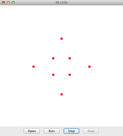
We have provided several modules, helper functions, test cases, and a
graphical interface that may be useful while developing your
solution. The function run_simulation
in Main_nbody can be used to generate "transcripts" of
simulations. The module Test_nbody defines the initial
values for several simulations. The Java
application bouncy.jar (depicted in the image above) can
be used to animate a simulations using a transcript.
Your Tasks
Your task for the first part of this problem is to implement the
naive n-body algorithm. In particular, you will need to
implement plane.ml and fill in the missing functions
in naive_nbody.ml.
To submit: plane.ml
and naive_nbody.ml.
The Barnes-Hut Algorithm (20pts)
The
Barnes-Hut
algorithm provides a way to approximate an n-body simulation,
while dramatically decreasing its cost. The insight behind the
algorithm is that the gravitational forces between objects separated
by large distances are weak, so they can be approximated without
affecting the fidelity of the overall simulation very much.
The algorithm works by grouping bodies into regions and
using a fixed threshold θ to determine if it should perform the
exact acceleration calculation for the each body in the
region, or if it should merely approximate acceleration
using a pseudobody that represents aggregate information about
all of the bodies contained in the region. This dramatically reduces
the time needed to perform large simulations — asymptotically,
from O(n^2) to O(n log n).
Bounding Boxes and Quad Trees
To represent regions, we will use bounding boxes comprising two
points:
type bbox = {north_west:Plane.point; south_east:Plane.point}
To represent the decomposition of a collection of bodies into regions,
we will use the following datatype:
type bhtree =
    Empty
  | Single of body
  | Cell of body * bbox * (bhtree Sequence.t)
Intuitively, Empty represents a region with no
bodies; Single(b) represents a region with a single
body b; and Cell(b,bb,qs) represents a
region with pseudobody b, bounding box bb,
and four sub-quadrants qs. The position of the pseudobody
in a Cell is the center of mass (or barycenter) of
all objects in the region. The mass of the pseudobody is the total
mass of all objects. The velocity of the pseudobody can be arbitrary,
as it is not needed for the acceleration calculation. In
your solution, you will likely have to write a function that
decomposes a sequence of n bodies into
a bhtree.
Simulation
The actual Barnes-Hut simulation works as follows. For each
body b, the algorithm traverses the top-level
bhtree. If it encounters a region with more than one body
— i.e., a Cell node — it checks
whether θ ≥ m / d, where m is the total mass
of the pseudobody associated with the region, and d is the
distance between b and the pseudobody's center of mass. If so,
then it treats the entire region as if it were one large
pseudobody. Otherwise, it recursively performs the computation on the
sub-quadrants of the region. The base cases are the Empty
and Single(b) cases, where the algorithm simply invokes
the acceleration function as in the naive algorithm.
Your Tasks
Your task for the second part of this problem is to implement the
Barnes-Hut algorithm. You will need to fill in the missing code
in barnes_hut_nbody.ml.
To submit: barnes_hut_nbody.ml.
Acknowledgments
This assignment is based on materials developed by Dan Licata
(Carnegie Mellon University) and Professor David Bindel.