
A graph
is a data structure consisting of a set of vertices, V, and a
set of edges, E. An edge e is a set of triples (u,
v, w) where u and v are the vertices connected
by e and w is the weight of e. A graph is
directed if we treat the edges as pointing from one vertex to another,
rather than just connecting them. For this problem, we will represent
a graph as the number of vertices in the graph, and a single list of
all the edges. A graph with the vertex set: {0, ..., n-1} and
edge set E consisting of k edges is represented by the
tuple: (n, [e_1; ... ;e_k]).
A minimum spanning tree of a graph is a subgraph whose edges connect every vertex and have least weight. Because this property is defined for undirected graphs, you should assume that edges point in both directions in the following discussion. If some vertices are unconnected, we will instead be interested in finding a collection of minimal spanning trees, one for each connected component.
Kruskal's algorithm is a greedy algorithm that computes a minimum spanning tree of a graph. It begins by constructing a graph containing the original vertices and no edges — that is is, each vertex is in its own trivially-connected component. Next, it orders the edges in the original graph in ascending order by weight. It then processes edges in order, adding it to the minimum spanning tree only if it connects two previously unconnected components. Once all edges have been processed, the resulting graph (all of the original vertices and the edges selected by the algorithm) is a minimum spanning tree, or a forest of minimum spanning trees if the original graph was not connected.
Many physical systems can be modeled using a percolation model. In this problem we will consider situations where the model comprises a simple 2-dimensional square grid and each square in the grid is either "occupied" or "vacant". The grid is said to percolate if the top and bottom of the grid are connected by vacant squares. This model is very flexible — depending on how "occupied" and "vacant" are defined, it can be used to represent a variety of systems. For example, to model social interaction, we can use vacant squares to represent people and occupied squares to represent nothing, so that percolation models communication. Another example is a model for electricity where a vacant site is a conductor, an occupied site is an insulator, and percolation means the material represented by a grid conducts electricity.
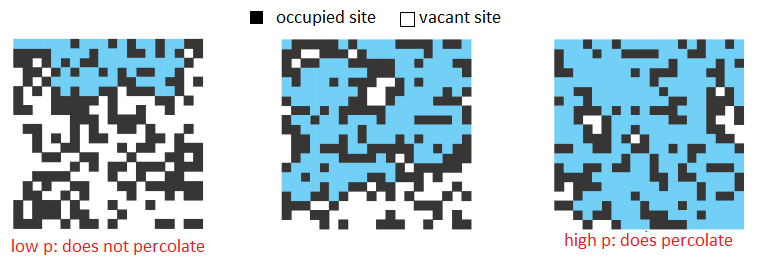
The likeliness of percolation depends on the site vacancy probability, p. Grids with low vacancy probability, are unlikely to percolate whereas grids with high vacancy probability are likely to percolate. A threshold p* has been discovered experimentally, such that a grid with p < p* almost certainly does not percolate, and a grid with p ≥ p* almost certainly does percolate. In this problem, you will estimate this percolation threshold p*. Interestingly, this percolation threshold p* is only known through simulation, and is approximately 0.592746 for large square lattices.
Your task will be to write a function calc_p_threshold
that takes an input
n representing is the size of the grid to use, and
returns an estimated percolation threshold p*. To do this, you
should:
n × n grid of occupied
squares. You may assume that n > 2.average_p_threshold
which runs calc_p_threshold multiple times for a grid of
the same size and averages the results of all of the runs.
In the provided part1.ml file, implement the
functions kruskal and calc_p_threshold
according to the specifications in the file and the above description.
We have provided an implementation of the disjoint set data
structure that you have seen in lecture, which you may find useful.
The name of the module is DisjointSet. The
file disjointSet.mli gives the signature for this module.
To submit: part1.ml.
|
|
sigma = 0.5, k = 500,
and min_size = 50.
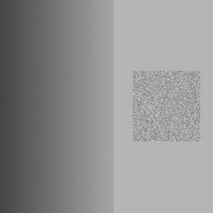
The goal of image segmentation is to partition an image into a set of perceptually important regions (sets of contiguous pixels). It's difficult to say precisely what makes a region "perceptually important" — in different contexts it could mean different things. You will implement an algorithm that uses the variation in pixel intensity as a way to distinguish perceptually important regions (also called segments). This simple criterion captures many intuitive notions of a segmentation quite well.
To illustrate how the algorithm uses intensity variation as a way to segment an image, consider the grayscale image below. The image on the right is the result you get from segmenting the image on the left. Each segment is given a white outline and given a solid color. All of the pixels in the large rectangular region on the right have the same intensity, so they are segmented together. The rectangular region on the left is considered its own segment because it is generally darker than the region on the right, and there is not much variation between the intensity of adjacent pixels. Interestingly, the noisy square on the right is considered a single region, because the intensity varies so much.
There are some large differences between the intensities of adjacent pixels in the small square region; larger even than the difference between pixels at the border of the two large rectangular regions. This tells us that we need more information than just the difference in intensity between neighboring pixels in order to segment an image.
Note that the algorithm found a few thin regions in the middle of the image. There is no inherent reason why these regions should be there; they were introduced as an artifact of smoothing the image, a process that will be discussed later.
 |
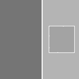 |
Parameters: sigma = 0.5, k = 500, min_size = 50.
Image segmentation provides you with a higher-level representation of the image. Often it is easier to analyze image segments than it is to analyze an image at the pixel level. For example, in the 2007 DARPA Urban Challenge, the Cornell vehicle detected road lines using this image segmentation algorithm. First, a camera in the front of the car takes a picture. Then the image is segmented using the algorithm you are going to implement. Since road lines look quite different from the road around them, they often appear as distinct segments. Each segment is then individually scored on how closely it resembles a road line, using a different algorithm.
Consider the image as a graph where each pixel corresponds to a
vertex. The vertex corresponding to each pixel is adjacent to the
eight vertices corresponding to the eight pixels surrounding it (and
no other vertices). Each edge has a weight, w(v1,
v2), defined as
 where ri, gi, bi
are the red, green, and blue components of pixel i
respectively.
where ri, gi, bi
are the red, green, and blue components of pixel i
respectively.
The image segmentation algorithm works by building a graph that contains a subset of these edges. We will start with a graph that contains all of the vertices but no edges. For each weighted edge, we will decide whether to add it to the graph or to omit it. At the end of this process, the connected components of the graph are taken to be the segments in the image segmentation (so we will refer to segments and connected components interchangeably).
We define the internal difference of a
connected component C as  where E(C) is the
set of edges that have been added to the graph between vertices in
C, and w(e) is the weight of e.
If C contains no edges, then define Int(C) =
0.
where E(C) is the
set of edges that have been added to the graph between vertices in
C, and w(e) is the weight of e.
If C contains no edges, then define Int(C) =
0.
Also define T(C) = k/|C|, where k is some fixed constant and |C| is the number of vertices in C. We call this the threshold of C.
At the beginning of the algorithm, there are no edges, so each vertex is its own connected component. So if the image is w by h pixels, there are w*h connected components. Sort the edges in increasing order. Now consider each edge {v1, v2} in order from least to greatest weight. Let C1 and C2 be the connected components that vertices v1 and v2 belong to respectively.
If C1 = C2, then omit the edge. Otherwise, add the edge if w(v1, v2) ≤ min(Int(C1) + T(C1), Int(C2) + T(C2)). This merges C1 and C2 into a single component.
Note that T(C) decreases rapidly as the size of C increases. For small components, Int(C) is small (in fact, it is 0 when |C| = 1). Thus Int(C) + T(C) is dominated by T(C) (the threshold) when C is small and then by Int(C) (the internal difference) when C is large. This reflects the fact that the threshold is most important for small components. As we learn more about the distribution of intensities in a particular component (information that is captured by Int(C)), the threshold becomes less important.
Once you have made a decision for each edge in the graph, take each connected component to be a distinct segment of the image.
You will find that the above algorithm produces a number of tiny, unnecessary segments. You should remove these segments once the algorithm is finished by joining small connected components with neighboring components. Specifically: order the edges that were omitted by the algorithm in increasing order. For each edge, if the components it joins are different, and one or both has size less than min_size, then add that edge to the graph. Call min_size the merging constant.
Before segmenting an image, you should smooth it using a Gaussian filter. Smoothing the image makes it less noisy and removes digitization artifacts, which improves segmentation. We have provided you with the code to do this, so you do not need to implement it yourself. Gaussian smoothing takes a parameter σ. The value σ = 0.8 seems to work well for this algorithm; larger values of σ smooth the image more.
We have provided you with a module called Image, that
provides functions for manipulating images. The module contains
functions for loading and saving bitmap files, Gaussian smoothing, and
a function for displaying images using the OCaml Graphics
library.
Your task is to implement the image segmentation algorithm
described above in the Segmentation module as three
separate functions: segmentGraph,
segmentImage, and
mergeSmallComponents.
segmentGraph function should take an arbitrary
graph with weighted edges as input and segment it using the above
algorithm (it should not matter that the graph does not correspond
to an image). This function should return a value of type
segmentation. You are free to define
segmentation however you like. To allow us to test your
code, you should write a function
components that takes a graph and a segmentation and
returns a list of components (i.e. segments). Each component will be
represented as a list of the integers corresponding to the vertices
in the component.mergeSmallComponents should take a
segmentation, a list of edges, and a merging threshold
min_size. It should merge segments whose size is less
than min_size as described above. Again, we will test
this function using the components function.segmentImage should take an image as
input and return a segmentation that partitions the
pixels in the image into segments. As discussed above, you should
smooth the image first (using Image.smooth), then build
a grid graph and segment it using segmentGraph and
merge small segments using mergeSmallComponents.
segmentImage should have complexity O(nlog(n)) where
n is the number of pixels in the image. Choose your data
structures carefully to achieve this. You may write imperative code
for this assignment.colorComponents should take an image
and its segmentation as input and return an image where the segments
are outlined and colored, like the one at the top of this
writeup. You should color any pixel that is adjacent to a pixel from
a different segment white (using the 8-neighbor definition for
adjacency described above). Then for each segment, compute the
average color of all of the pixels in that segment (i.e. by
separately computing the average red, green, and blue components of
the colors in that segment), and assign this color to every pixel
that is not a border pixel. Although this algorithm sounds complicated, you should not need to
write much code. Our solution is less than 150 lines of code. For
convenience, we have provided you with a function called
Segmentation.segmentAndShow that segments a bitmap
file, colors it using colorComponents, shows you the
result, and saves the result as segmented.bmp.
Note: The results of your algorithm may be slightly different from the examples given here, because the order that you consider the equal-weight edges influences the segmentation. In other words, after you sort your edges by weight, if you then permute the edges with equal weight, you may get different results.
To submit: segmentation.ml.
If you would like to define additional modules, please put them inside the file segmentation.ml. This will make it easier to test your code.
Any functions or modules defined in segmentation.ml will be
available in the Segmentation module. For example, if
you define a module named Foo in segmentation.ml,
it can be used as Segmentation.Foo.
This phenomenon occurs because when you compile OCaml code using
ocamlc, each file you compile automatically defines a module. For
example, functions defined in foo.ml are automatically placed
into a module called Foo without using the module
Foo = construct.
You should build a custom toplevel containing all of your PS4 code,
from part 1, part 2 and the karma problem. We have provided a script
called buildToplevel.bat (or buildToplevel.sh for Unix) which creates
such a toplevel. To start the toplevel, execute the script
runToplevel.bat (or runToplevel.sh). ThePart1,
Image and Segmentation modules
will automatically be loaded.
Prove the following statements using the inference rules provided in the lecture on natural deduction (don't use any of the tautologies).

Prove the following statements using the inference rules for propositional and predicate logic in Lectures 13 and 14. Note that P, Q are predicates.
Submit a file logic.txt or logic.pdf containing your solutions.
Prove the following additional statements:


Several algorithms, including compression algorithms and string matching algorithms, make use of maps where the keys are sequences of values of a certain type. A trie or prefix tree is an efficient data structure for implementing the map ADT for this kind of map. The set of elements from which key sequences are built is called the alphabet of the trie.
A trie is a tree structure whose edges are labeled with the elements of the alphabet. Each node can have up to N children, where N is the size of the alphabet. Each node corresponds to the sequence of elements traversed on the path from the root to that node. The map binds a sequence s to a value v by storing the value v in the node corresponding to s. The advantage of this scheme is that it efficiently represents common prefixes, and lookups or inserts are achieved using quick searches starting from the root.
Suppose we want to build a map from lists of integers to strings. In this case, edges are labeled with integers, and strings are stored in (some of) the nodes. Here is an example:

The above trie describes the map {[2; 3]->"zardoz", [2; 3; 2]->"cow",
[5; 4]->"test", [5; 9]->"hello"}. The values are stored
in the nodes. Note that not all nodes have values. For instance, the node
that corresponds to the list [5] has no value. Hence,
[5] is not in the map.
Your mission, should you choose to accept it, is to implement a trie, and then use it to sort of list of strings in lexicographical order. The sorting function must have O(n) complexity, where n is the sum of the lengths of the strings (assuming the alphabet is of constant size).
To submit: trie.ml.