|
|
sigma = 0.5, k = 500,
and min_size = 50.
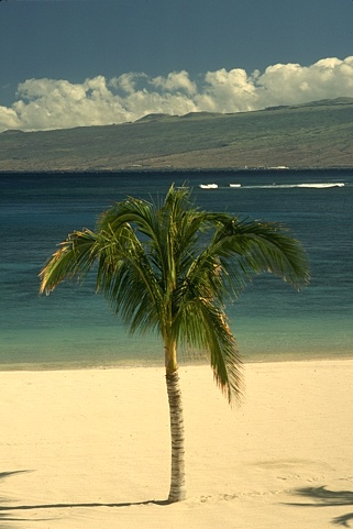
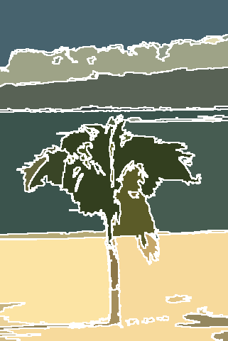
The goal of image segmentation is to partition an image into a set of perceptually important regions (sets of contiguous pixels). It's difficult to say precisely what makes a region "perceptually important", and in different contexts it could mean different things. The algorithm you are going to implement uses the variation in pixel intensity as a way to distinguish perceptually important regions (also called segments). This criterion seems to capture our intuitive notion of a segmentation quite well.
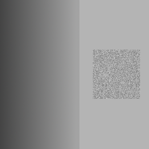
To illustrate how the algorithm uses intensity variation as a way to segment an image, consider the grayscale image below. The image on the right is the result you get from segmenting the image on the left. Each segment is given a white outline and given a solid color. All of the pixels in the large rectangular region on the right have the same intensity, so they are segmented together. The rectangular region on the left is considered its own segment because it is generally darker than the region on the right, and there is not much variation between the intensity of adjacent pixels. Interestingly, the noisy square on the right is considered a single region, because the intensity varies so much.
There are some large differences between the intensities of adjacent pixels in the small square region; larger even than the difference between pixels at the border of the two large rectangular regions. This tells us that we need more information than just the difference in intensity between neighboring pixels in order to segment an image.
Note that the algorithm found a few thin regions in the middle of the image. There is no good theoretical reason why these regions should be there: they were simply introduced as an artifact of smoothing the image, a process that will be discussed later.
 |
 |
Parameters: sigma = 0.5, k = 500, min_size = 50.
Image segmentation provides you with a higher-level representation of the image. Often it is easier to analyze image segments than it is to analyze an image at the pixel level. For example, in the 2007 DARPA Urban Challenge, Cornell's vehicle detected road lines using this image segmentation algorithm. First, a camera in the front of the car takes a picture. Then the image is segmented using the algorithm you are going to implement. Since road lines look quite different from the road around them, they often appear as distinct segments. Each segment is then individually scored on how closely it resembles a road line, using a different algorithm.
Consider the image as a graph where each pixel corresponds to a
vertex. The vertex corresponding to each pixel is adjacent to the
eight vertices corresponding to the eight pixels surrounding it (and
no other vertices). Each edge has a weight, w(v1,
v2), defined to be
 where ri,
gi, bi are the red, green, and blue components
of pixel i respectively.
where ri,
gi, bi are the red, green, and blue components
of pixel i respectively.
The image segmentation algorithm works by building a graph that contains a subset of these edges. We will start with a graph that contains all of the vertices but no edges. For each weighted edge, we will decide whether to add it to the graph or to omit it. At the end of this process, the connected components of the graph are taken to be the segments in the image segmentation (so we will refer to segments and connected components interchangeably).
We define the internal difference of a
connected component C to be  where
where E(C) is the
set of edges that have been added to the graph between vertices in
C, and w(e) is the weight of e.
If C contains no edges, then define Int(C) =
0.
Also define T(C) = k/|C|, where k is some
fixed constant and |C| is the number of vertices in C.
We call this the threshold of C.
At the beginning of the algorithm, there are no edges, so each
vertex is its own connected component. So if the image
is w by h pixels, there are
w*h connected components. Sort the edges in
increasing order. Now consider each edge
{v1, v2} in order from
least to greatest weight. Let C1
and C2 be the connected components that
vertices v1 and v2 belong to respectively.
If C1 = C2, then omit the edge.
Otherwise, add the edge if
w(v1, v2) ≤ min(Int(C1) +
T(C1), Int(C2) + T(C2)).
This merges C1
and C2 into a single component.
Note that T(C) decreases rapidly as the size
of C increases. For small
components, Int(C) is small (in fact, it is 0
when |C| = 1). Thus Int(C) + T(C) is
dominated by T(C) (the threshold) when C
is small and then by Int(C) (the internal difference)
when C is large. This reflects the fact that the
threshold is most important for small components. As we learn more
about the distribution of intensities in a particular component
(information that is captured by Int(C)), the threshold
becomes less important.
Once you have made a decision for each edge in the graph, take each connected component to be a distinct segment of the image.
You will find that the above algorithm produces a number of tiny,
unnecessary segments. You should remove these segments once the
algorithm is finished by joining small connected components with
neighboring components. Specifically: order the edges that were
omitted by the algorithm in increasing order. For each edge, if the
components it joins are different, and one or both has size less
than min_size, then add that edge to the graph.
Call min_size the merging constant.
Before segmenting an image, you should smooth it using a Gaussian filter. Smoothing the image makes it less noisy and removes digitization artifacts, which improves segmentation. We have provided you with the code to do this, so you do not need to implement it yourself. Gaussian smoothing takes a parameter σ. The value σ = 0.8 seems to work well for this algorithm; larger values of σ smooth the image more.
We have provided you with a module called Image,
which provides functions for manipulating images. The module
contains functions for loading and saving bitmap files,
Gaussian smoothing, and a function for displaying images using
the OCaml Graphics
library.
Please implement the image segmentation algorithm described
above in the Segmentation module as three
separate functions: segment_graph,
segment_image, and
merge_small_segments.
segment_graph should take an arbitrary graph
with weighted edges as input and segment it using the above
algorithm (it should not matter that the graph does not correspond
to an image). This function should return a value of type
segmentation. You are free to define
segmentation however you like. However, we will still
need to test your code. Thus you should write a function
segments which takes a graph and a segmentation and
returns a list of components (i.e. segments). Each component will be
represented as a list of the integers corresponding to the vertices
in the component.
merge_small_segments should take a
segmentation, a list of edges, and a merging threshold
min_size. It should merge segments whose size is less
than min_size as described above. Again, we will test
this function using the segments function.
segment_image should take an image as input and
return a segmentation that partitions the pixels in the
image into segments. As discussed above, you should smooth the image
first (using Image.smooth), then build a grid graph and
segment it using segment_graph and merge small segments
using merge_small_segments.
segment_image should have complexity O(nlog(n))
where n is the number of pixels in the image. Choose your data
structures carefully to achieve this runtime. You may write
imperative code for this assignment.
color_segments should take an image and its
segmentation as input and return an image where the segments are
outlined and colored, like the one at the top of this writeup. You
should color any pixel that is adjacent to a pixel from a different
segment (using the 8-neighbor definition for adjacency described
above). Then for each segment, compute the average color of all of
the pixels in that segment (i.e. by separately computing the average
red, green, and blue components of the colors in that segment), and
assign this color to every pixel that is not a border pixel. Segmentation.segment_and_show that segments a bitmap
file, colors it using color_segments, shows you the
result, and saves the result as segmented.bmp.
Note: The results of your algorithm may be slightly
different from the examples given here, because the order that you
consider the equal-weight edges influences the segmentation. In
other words, after you sort your edges by weight, if you then
permute the edges with equal weight, you may get different
results.
To submit: segmentation.ml.
You will build a custom toplevel containing all of your PS4
code. We have provided a script called buildToplevel.bat (or
buildToplevel.sh for Unix) which creates such a toplevel. To start the
toplevel, execute the script runToplevel.bat (or runToplevel.sh). The
Image and Segmentation modules will
automatically be loaded.
If you would like to define additional modules, please put them in segmentation.ml. This will make it easier to test your code.
Any functions or modules defined in segmentation.ml will be
available in the Segmentation module. For example, if
you define a module named Foo in segmentation.ml,
it will be known as Segmentation.Foo.
This phenomenon occurs because when you compile OCaml code using
ocamlc, each file you compile automatically defines a module. For
example, functions defined in foo.ml are automatically placed
into a module called Foo without using the module Foo
= construct.
For this part of the assignment, you will an AA-tree, a type of balanced binary search tree, to implement a key-value map. An AA-tree satisfies the following invariants in addition to the binary tree invariants:
Each node has an integer associated with it called a level, which roughly (not exactly) corresponds to the depth of the tree rooted at that node. The level serves a function somewhat analogous to the colors in a red-black tree. As the definition states, leaf nodes all have level 1, while the level of a parent node is strictly greater than that of its left child and greater than or equal to that of its right child. A node must always have a greater level than its grandchild. In addition, the regular Binary Search Tree invariant holds. For any node, all nodes in the left sub-tree should have values less than that node and all nodes on the right sub-tree should have values greater than or equal to the value of that node.
To keep an AA-tree balanced, you need to test the levels and make sure that none of the invariants are broken. If an invariant is broken, then you need to fix the levels while keeping the relationships between the values in the nodes intact. Rebalancing can be broken into two operations called skew and split.
Skew is used when you encounter a situation where a node has the same level as its left child, breaking the invariant. Skew essentially rotates the tree so that the relationships between the values stay the same, but the nodes are rearranged so that the level equality is now on the right (which is allowed). Note that no changes are needed to the levels after a skew because the operation simply turns a left level equality into a right level equality. An example is shown (letters are the values, numbers are the levels):
         d,2               b,2
        /   \             /   \
     b,2     e,1  -->  a,1     d,2
    /   \                     /   \
 a,1     c,1               c,1     e,1
Split removes two consecutive level equalities on the right by rotating left and increasing the level of the parent. A split needs to change the level of a single node because if a skew is made first, a split will negate the changes made by doing the inverse of a skew. Therefore, a proper split will force the new parent to a higher level:
     b,2                     d,3
    /   \                  /     \
 a,1     d,2     -->     b,2      f,2
        /   \           /  \      /  \
     c,1     f,2     a,1   c,1  e,1  g,1
	     /  \
           e,1  g,1
It is important to note that one should do skew before split, because a skew operation can result in a tree that requires a split:
     5,1         4,1                5,2
    /   \    -->    \       -->    /   \
 4,1     6,1         5,1        4,1     6,1
                        \
                         6,1
After any insertion or removal, the tree needs to be checked for level equalities on the left (which need to be fixed by skews), and then for two or more consecutive level equalities on the right (which need to be fixed by splits).
For this assignment, you need to implement an AA-tree for use as a dictionary which fits the provided signature. This means you need to implement the following, all of which are specified in the signature:
emptyinsertremovefindfoldto_listThe fold function should do an in-order traversal of the tree, and the to_list function should run in O(n) time.
The dictionary needs to work for any type of comparable key, so you will also need to implement support for a functor which defines the key type and a comparison function. The signature for this functor is also provided. We will not require you to submit an implementation of this signature, but you will obviously need to write an implementation of your own to test the functor support of your AA-tree module.
We will also require you to write a repOK function. The repOK function should take an AA-tree and return back the same tree unchanged if the tree is a valid AA-tree. If the tree is invalid it should throw an exception. It would be a good idea to implement this early on for use as a debugging tool in writing the other functions (because you can just use repOK on the result of the function before returning to make sure the function returns a valid AA-tree). Take out the debug uses of repOK before submitting, though.
Along with the signatures, you are given a stub file to help you start writing your implementation. The stub file includes the following:
skew and split
functions, which must be implemented using the given signatures if
you want to use fix. We suggest you implement
skew and split in some form for use in the
insert method.fix method. This method is
for use in the remove method.
For the remove method, you are given a function fix which will rebalance
a tree as per the AA-tree invariants. You are free (but not required) to use this
function in the remove method so you do not have to reason about the order of
skews and splits. However, for fix to work, you need to call it on every
sub-tree which may have a balancing issue, so you will need to figure out where to
put it in order to take advantage of the code. fix
in the insert method.
In addition to implementing the required methods, you need to add the module definition, complete with the functor, and then define the key type appropriately. All you need to hand in is the completed implementation as specified here.
To submit: aatree.ml
Prove the following statements using the inference rules provided in the lecture on natural deduction (don't use any of the tautologies).
Prove the following statements using the inference rules for propositional logic and quantifiers presented in lecture. Note that p, q are names of predicates.