Problem Set 4: Image Segmentation

Due 3/19

For this problem set, you are to turn in an overview document covering parts 1 and 2. The overview document should be composed as described in Overview Requirements. You should read this document carefully. We have provided an example overview document written as if for Problem Set 2 from CS 312, Spring 2008. Submission in PDF is preferred; however, you can also submit your overview document as a .doc or a .txt file.

In particular, starting with this problem set, it's your job to convince us that your code works, by describing your implementation and by presenting a testing strategy, test cases, and results.

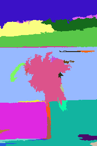
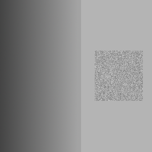
Example: sigma = 0.5, k = 500, and minSize = 50.

Part 1: Graph-based Image Segmentation (55 points)

The idea:

The goal of image segmentation is to partition an image into a set of perceptually important regions (sets of contiguous pixels). It's difficult to say precisely what makes a region "perceptually important", and in different contexts it could mean different things. The algorithm you are going to implement uses the variation in intensity as a way to distinguish perceptually important regions (also called segments). This criteria seems to capture our intuitive notion of a segmentation quite well.

To illustrate how the algorithm uses intensity variation as a way to segment an image, consider the grayscale image below. The image to its right was obtained by applying the image segmentation algorithm and then randomly coloring the segments. All of the pixels in the large rectangular region on the right have the same intensity, and so they are segmented together. The rectangular region on the left is considered its own segment because it is generally darker than the region on the right, and there is not much variation between the intensity of adjacent pixels. Interestingly, the noisy square on the right is considered a single region, because the intensity varies so much.

There are some large differences between the intensities of adjacent pixels in the small square region; larger even than the difference between pixels at the border of the two large rectangular regions. This tells us that we need more information than just the difference in intensity between neighboring pixels in order to segment an image.

Note that the algorithm found a few thin regions in the middle of the image. There is no good theoretical reason why these regions should be there: they were simply introduced as an artifact of smoothing the image, a process that will be discussed later.

Parameters: sigma = 0.5, k = 500, minSize = 50.

Image segmentation provides you with a higher-level representation of the image. Often it is easier to analyze image segments than it is to analyze an image at the pixel level. For example, in the 2007 DARPA Urban Challenge, Cornell's vehicle detected road lines using this image segmentation algorithm. First, a camera in the front of the car takes a picture. Then the image is segmented using the algorithm you are going to implement. Since road lines look quite different from the road around them, they often appear as distinct segments. Each segment is then individually scored on how closely it resembles a road line, using a different algorithm.

The Algorithm

Consider the image as a graph where each pixel corresponds to a vertex. The vertex corresponding to each pixel is adjacent to the eight vertices corresponding to the eight pixels surrounding it (and no other vertices). Each edge has a weight, w(v₁, v₂), defined to be where r_i, g_i, b_i are the red, green, and blue components of pixel i respectively.

The image segmentation algorithm works by building a graph that contains a subset of these edges. We will start with a graph that contains all of the vertices but no edges. For each weighted edge, we will decide whether add it to the graph or omit it. At the end of this process, the connected components of the graph are taken to be the segments in the image segmentation.

We define the internal difference of a connected component C to be where E(C) is the set of edges that have been added to the graph between vertices in C, and w(e) is the weight of e. If C contains no edges, then define Int(C) = 0.

Also define T(C) = k/|C|, where k is some fixed constant and |C| is the number of vertices in C. We call this the threshold of C.

At the beginning of the algorithm, there are no edges, so each vertex is its own connected component. So if the image is w by h pixels, there are w*h connected components. Sort the edges in increasing order. Now consider each edge {v₁, v₂} in order from least to greatest weight. Let C₁ and C₂ be the connected components that vertices v₁ and v₂ belong to respectively.

If C₁ = C₂, then omit the edge. Otherwise, add the edge if w(v₁, v₂) ≤ min(Int(C₁) + T(C₁), Int(C₂) + T(C₂)). This merges C₁ and C₂ into a single component.

Note that T(C) decreases rapidly as the size of C increases. For small components, Int(C) is small (in fact, it is 0 when |C| = 1). Thus Int(C) + T(C) is dominated by T(C) (the threshold) when C is small and then by Int(C) (the internal difference) when C is large. This reflects the fact that the threshold is most important for small components. As we learn more about the distribution of intensities in a particular component (information that is captured by Int(C)), the threshold becomes less important.

Once you have made a decision for each edge in the graph, take each connected component to be a distinct segment of the image.

Merging small components

You will find that the above algorithm produces a number of tiny, unnecessary segments. You should remove these segments once the algorithm is finished by joining small connected components with neighboring components. Specifically: order the edges that were omitted by the algorithm in increasing order. For each edge, if the components it joins are different, and one or both has size less than minSize, then add that edge to the graph. Call minSize the merging constant.

Smoothing

Before segmenting an image, you should smooth it using a Gaussian filter. Smoothing the image makes it less noisy and removes digitization artifacts, which improves segmentation. We have provided you with the code to do this, so you do not need to implement it yourself. Gaussian smoothing takes a parameter σ. The value σ = 0.8 seems to work well for this algorithm; larger values of σ smooth the image more.

Your task:

We have provided you with a module called Image, which provides functions for manipulating images. The module contains functions for loading and saving bitmap files, Gaussian smoothing, and a function for displaying images using the OCaml standard Graphics library.

To make your code easier to test, you should implement the image segmentation described above in the Segmentation module as three separate functions: segmentGraph, segmentImage, and mergeSmallComponents.

segmentGraph should take an arbitrary graph with weighted edges as input and segment it using the above algorithm (it should not matter that the graph does not correspond to an image). This function should return a value of type graph_segmentation. You are free to define graph_segmentation however you like. However, we will still need to test your code. Thus you should write a function components which takes a graph and a graph_segmentation and returns a list of components. Each component will be represented as a list of int corresponding to the vertices in the component.
mergeSmallComponents should take a graph_segmentation, a list of edges, and a merging threshold minSize. It should merge components whose size is less than minSize as described above. Again, we will test this function using the components function.
segmentImage should take an image as input and return a new image such that each segment of the original image is assigned random color. As discussed above, you should smooth the image first (using Image.smooth), then build a grid graph and segment it using segmentGraph and merge small components using mergeSmallComponents. Then create a new image and color the components. This function should have complexity O(nlog(n)) where n is the number of pixels in the image. Choose your data structures carefully to achieve this runtime. You may write imperative code for this assignment.

Though this algorithm sounds complicated at first glance, you should not need to write much code. Our solution is 135 lines of code.

Note: The results of your algorithm may be slightly different from the examples given here, because the order that you consider the equal-weight edges influences the segmentation. In other words, after you sort your edges by weight, if you then permute the edges with equal weight, you may get different results.

To submit: segmentation.ml.

Building and running your code

You will build a custom toplevel containing all of your PS4 code. We have provided a script called buildToplevel.bat (or buildToplevel.sh for Unix) which creates such a toplevel. To start the toplevel, execute the script runToplevel.bat (or runToplevel.sh). The Image and Segmentation modules will automatically be loaded.

Modules

If you would like to define additional modules, please put them in segmentation.ml. This will make it easier to test your code.

Any functions or modules defined in segmentation.ml will be available in the Segmentation module. For example, if you define a module named Foo in segmentation.ml, it will be known as Segmentation.Foo. You may need to modify segmentation.mli to make it accessible from the toplevel, though.

This phenomenon occurs because when you compile OCaml code using ocamlc, each file you compile automatically defines a module. For example, functions defined in foo.ml are automatically placed into a module called Foo without using the module Foo = construct.

Part 2: AVL Trees (30 points)

AVL trees were invented by Adelson-Velskii and Landis in 1962. An AVL tree is a balanced binary search tree where every node in the tree satisfies the following invariant: the height difference between its left and right children is at most 1. Hence, all sub-trees of an AVL tree are themselves AVL. The height difference between children (either the height of the left child minus that of the right or vice versa) is referred to as the balance factor of the node.

In this part of the assignment you will implement a map abstraction using an AVL tree. The AVL tree set is a functor parameterized on a signature ORD_BIND containing the types of keys and values and function that compares two keys. Each node of the tree contains an element and the height of the current node. The type definition of the AVL tree map is as follows:

type 'a avl = Empty | Node of height * key * 'a * 'a avl * 'a avl

Your task is to write the following functions:

Write repOK. Implement a repOK function that checks whether a tree is a valid AVL tree map. For full score, your implementation must be O(n) in the number of nodes of the tree. We suggest implementing repOK first, because it is useful for testing the rest of your functions.
balance: Implement the rebalancing function for AVL trees (described below). The argument of this function is a tree whose balance factor is between -2 and 2, and all subtrees are AVL trees. It returns an AVL tree that contains the same bindings as the given tree.
Write add and remove. Implement these operations using the balancing function, balance. The code you write for these functions should be very similar to add and remove for an unbalanced AVL tree, with the addition of some calls to balance.
You should state the representation invariant and abstraction function for your AVL tree.

To give you an estimate of how many lines of code your solution should be: our solution is roughly 130 lines of code.

Balancing an AVL Tree

The balance function should work by doing tree rotations. This is a reorganizing of the tree in which the parent-child relationships between nodes are changed in a local way, usually to restore a global invariant. There are two basic tree rotations, left rotations and right rotations, which are symmetrical. A left rotation works as follows, moving the root node to the left:

     x                       y
   /   \                   /   \
  +     y                 x     +
 /a\   / \       ===>    / \   /c\
 ---  +   +             +   +  ---
     /b\ /c\           /a\ /b\
     --- ---           --- ---

A right rotation is just the inverse transformation. The important property is that tree rotations preserve the BST invariant, because the left-to-right ordering of all nodes remains unchanged: x < a < b < y < c Therefore tree rotations can be used to reestablish other invariants such as the AVL invariant.

The balance function is invoked on a node t that is possibly unbalanced. We assume that whatever operation has been performed on the tree below this node, it has changed the height of nodes by at most one, and therefore the child subtrees of t have a height difference of at most 2. We also assume the subtrees satisfy the AVL invariant themselves. If the height difference (balance factor) is 1 or 0, then balance doesn't need to do anything. Suppose the balance factor is 2 (the case where it is −2 is symmetrical). Then the tree t looks something like this:

           y
        /     \
       +       +
      / \     / \
     /   \   / h \
    / h+2 \  -----
   /       \
   ---------

How we fix this problem depends on what the left subtree looks like. There are two cases to consider:

        Case 1                    Case 2

           y                         y
        /     \                   /     \
       x       +                 x       z
     /   \    /h\              /   \    /h\
    +     +   ---             +     +   ---
   / \   / \   c             /h\   / \   c
  /h+1\ /h+1\                ---  /h+1\
  ----- -----                 a   -----
    a     b (may be h)              b

In Case 1, we can do a right rotation to pull the subtrees a and b up:

Case 1:
          y                         x
	/   \                     /   \
       /     \                   /     \
      x       +                 +        y
    /   \    /h\     ====>     / \     /   \
   +     +   ---              /h+1\   +     +
  / \   / \   c               -----  / \   /h\
 /h+1\ /h+1\                    a   /h+1\  ---
 ----- -----                        -----   c
   a     b (may be h)                 b

This clearly wouldn't work if the height of subtree a were h, because in that case b's leaves would be two levels lower than a's. That's the job of Case 2, which requires a double rotation:

Case 2:
       z                  y
     /   \              /   \
    /     \            /     \
   x       +          x        z
  /  \    /h\ ====>  / \      / \
 +    y   ---       +   +    +   +
/h\  / \   c       /h\ /h\  /h\ /h\
--- +   +          --- ---  --- ---
 a /h\ /h\          a   b'  b''  c
   --- ---
    b'  b''

(Note that one of b' or b'' can actually have height h−1 here, but that doesn't break the AVL invariant). The double rotation preserves the BST ordering because it is equivalent to two rotations. So the ordering remains unchanged: a < x < b' < y < b'' < z < c

To submit: avl.ml

Part 3: Induction (15 points)

A tree is a connected graph with no cycles in it. Equivalently, it is a connected graph with exactly N-1 edges, where N is the number of nodes. The diameter of a tree is the maximum distance between some pair of two nodes. It turns out that there is a simple algorithm for finding the diameter of a tree:

Pick an arbitrary node, call it u.
Run BFS (or DFS) to find the nodes furthest from u. Of all the nodes furthest from u, pick one arbitrarily, call it v.
Run BFS (or DFS) to find the nodes furthest from v. The distance from v to the furthest node from v is the diameter of the tree.

Prove that this algorithm correctly finds the diameter of a tree.

To submit: induction.txt or induction.pdf.

Stack language (Karma)

In this part you will use higher-order functions to implement a simple stack language that computes on integers. Note: this is tricky! The commands in this language are:

`start`	Initializes the stack to empty. This is always the first command and never appears again.
`(push n)`	Pushes the integer n on the top of the stack. This command is always parenthesized with its argument.
`pop`	Removes the top element from the stack.
`add`	Pops the two top elements and pushes their sum.
`mul`	Pops the two top elements and pushes their product.
`npop`	Pops the top element, elt, and if elt is positive, pops elt more elements
`dup`	Duplicates the top element and pushes it.
`halt`	Terminates execution. This is always the last command.

Remarkably, we can implement each of the commands as OCaml functions, in a way that lets us write a series of stack-language commands directly as OCaml expressions. The value of the OCaml expression should be the final stack configuration. For example, the following series of commands:

start (push 2) (push 3) (push 4) mul mul halt

evaluates to a stack with one element, 24. Note: this is actual OCaml code!

Your task is to implement all of the commands in this language. Use a list to implement the stack such that the previous example returns the stack [24], and raise the provided StackException if a command cannot be performed on the current stack, e.g. the command add in the program start add halt.

Sorting (Karma)

Use the trie you wrote in PS3 to implement a function sort : string list -> string list that sorts a list of strings in lexicographical order. It must have O(n) complexity, where n is the sum of the lengths of the strings.