
Suppose we want a data structure to implement either a set of
elements with operations like contains, add, and remove that take an element
as an argument, or a map (function) from keys to values with operations like get,
put, and remove that take a key or a (key,value) pair for an argument. A map
represents a partial function that maps keys to values; it is partial because it is not defined on all keys,
but only on those that have been put into the map. We have now seen a few data structures that could
be used for both of these implementation tasks.
We consider the problem of implementing sets and maps together, because most data structures that can implement a set can also implement a map and vice versa. A set of (key,value) pairs can act as a map, provided there is at most one (key,value) pair in the map with a given key. Conversely, a map that maps every key to a fixed dummy element can be used to represent a set of keys.
Here are the data structures we've seen so far, with the asymptotic complexities for each of their operations:
| Data structure | lookup (contains/get) | add/put | remove |
|---|---|---|---|
| Array | O(n) | O(1) | O(n) |
| Sorted array | O(lg n) | O(n) | O(n) |
| Linked list | O(n) | O(1) | O(n) |
| Balanced search tree | O(lg n) | O(lg n) | O(lg n) |
Naturally, we might wonder if there is a data structure that can do better. And it turns out that there is: the hash table, one of the best and most useful data structures there is—when used correctly.
Many variations on hash tables have been developed. We'll explore the most common ones, building up in steps.
While arrays make a slow data structure when you don't know what index to look at, all of their operations are very fast when you do. This is the insight behind the direct address table. Suppose that for each element that we want to store in the data structure, we can determine a unique integer index in the range \(0\dots m-1\). That is, we need an injective function that maps elements (or keys) to integers in the range. Then we can use the indices produced by the function to decide at which index to store the elements in an array of size \(m\).
For example, suppose we are maintaining a collection of objects representing houses on the same street. We can use the street address as the index into a direct address table. Not every possible street address will be used, so some array entries will be empty. This is not a problem as long as there are not too many empty entries.
However, it is often hard to come up with an injective function that does not require many empty entries. For example, we might try to maintain a collection of employees along with their social security numbers, and to look them up by social security number. Using the social security number as the index into a direct address table would require an array of 10 billion elements, almost all of which are likely to be unused. Even assuming our computer has enough memory to store such a sparse array, it will be a waste of memory. Furthermore, on most computer hardware, the use of caches means that accesses to large arrays are actually significantly slower than accesses to small arrays, sometimes by two orders of magnitude.
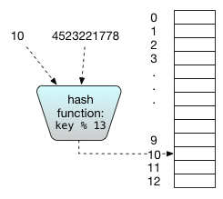
Instead of requiring that each key be mapped to a unique index, hash tables allow a collisions in which two keys maps to the same index, and consequently the array can be smaller, on the order of the number of elements in the hash table. The entries in the array are called buckets, and we use \(m\) to denote the number of buckets. The mapping from keys to bucket indices is performed by a hash function; it maps the key in a reproducible way to a hash value that is a legal array index.
If the hash function is good, it will distribute the values fairly evenly, so that collisions occur infrequently, as if at random. In particular, what we want from the hash function is that for any two different keys generated by the program, the chance that they collide is approximately \(1/m\).For example, suppose we are using an array with 13 entries and our keys are
social security numbers. Then we might use modular hashing, in which
the array index is computed as (key % 13). Modular hashing is not
very random, but is likely to be good enough in many applications.
In some applications, the keys may be generated by an adversary, who is purposely choosing keys that collide. In this case, the choice of hash function must be made carefully to prevent the adversary from engineering collisions. Modular hashing will not be good enough. A cryptographic hash function should be used so that the adversary cannot produce collisions at a rate higher than random choice.
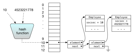
There are two main ideas for how to deal with collisions. The best way is usually chaining: each array entry corresponds to a bucket containing a mutable set of elements. (Confusingly, this approach is sometimes known as closed addressing or open hashing.) Typically, the bucket is implemented as a linked list, and each array entry (if nonempty) contains a pointer to the head of the list. The list contains all keys that have been added to the hash table that hash to that array index.
To check whether an element is in the hash table, the key is first hashed to find the correct bucket to look in, then the linked list is scanned for the desired element. If the list is short, this scan is very quick.
An element is added or removed by hashing it to find the correct bucket. Then, the bucket is checked to see if the element is there, and finally the element is added or removed appropriately from the bucket in the usual way for linked lists.
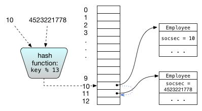
Another approach to collision resolution is probing. (Equally confusingly, this technique is also known as open addressing or closed hashing.) Rather than put colliding elements in a linked list, all elements are stored in the array itself. When adding a new element to the hash table creates a collision, the hash table finds somewhere else in the array to put it. The simple way to find an empty index is to search ahead through the array indices with a fixed stride (usually 1) for the next unused array entry, wrapping modulo the length of the array if necessary. This strategy is called linear probing. It tends to produce a lot of clustering of elements, leading to poor performance. A better strategy is to use a second hash function to compute the probing interval; this strategy is called double hashing.
Regardless of how collisions are resolved, the time required for the hash table operations grows as the hash table fills up. By contrast, the performance of chaining degrades more gracefully, and chaining is usually faster than probing even when the hash table is not nearly full. Therefore chaining is often preferred over probing.
A recently popular variant of closed hashing is cuckoo hashing, in which two hash functions are used. Each element is stored at one of the two locations computed by these hash functions, so at most two table locations must be consulted in order to determine whether the element is present. If both possible locations are occupied, the newly added element displaces the element that was there, and this element is then re-added to the table. In general, a chain of displacements occurs.
Suppose we are using a chained hash table with m buckets, and the number of elements in the hash table is n. The average number of elements per bucket is n/m, which is called the load factor of the hash table, denoted α. When we search for an element that is not in the hash table, the expected length of the linked list traversed is α. If the hash function is indistinguishable from a random function, the probability distribution of the length of the longest linked list falls off exponentially in the list length, so the longest bucket length is \(O(α)\). Since even when \(α\) is small, there is always at least some \(O(1)\) cost of hashing, the cost of hash table operations with a good hash function is, on average, \(O(1 + α)\). If we can ensure that the load factor α never exceeds some fixed value \(α_{max}\), then all operations take \(O(1 + α_{max}) = O(1)\) time on average and, if the hash function is random, in the worst case.
In practice, we will get the best performance out of hash tables when α is within a narrow range, from approximately 1/2 to 2. If α is less than 1/2, the bucket array is becoming sparse and a smaller array is likely to give better performance. If α is greater than 2, the cost of traversing the linked lists limits performance. The optimal bounds on α depend on details of the architecture; these days it is common to keep α between 1/2 and 1.
One way to hit the desired range for α is to allocate the bucket array to just the right size for the number of elements that are being added to it. In general, however, it's hard to know ahead of time what this size will be, and in any case, the number of elements in the hash table may need to change over time.
Since we cannot predict how big to make the bucket array ahead of time, we can use a resizable array to dynamically adjust the size when necessary. Instead of representing the hash table as a bucket array, we introduce a hash table object that maintains a pointer to the current bucket array and the number of elements that are currently in the hash table.
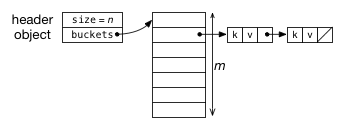
If adding an element would cause α to exceed α_{max}, the hash table generates a new bucket array whose size is a multiple of the current size, usually twice the size. This means the hash function must change, so all the elements must be rehashed into the new bucket array. Hash functions are typically designed so they take the array size m as a parameter, so this parameter just needs to be changed.
Resizable arrays are also used to implement variable-length array
abstractions like ArrayList, because its size can be
changed at run time.
With the above procedure, some add operations will cause
all the elements in the hash table to be rehashed. We have to search
the array for the nonempty buckets, hash all the elements, and add
them to the new table. This will take time \(O(n)\)
(provided \(n\) is at least a constant fraction of the
size of the array). For a large hash table, this may take enough time
that it causes problems for the program. Perhaps surprisingly, however,
the expected cost per operation is still \(O(1)\). In
particular, any sequence of n operations on the hash table always takes
expected time \(O(n)\), or \(O(1)\)
per operation. Therefore we say that the amortized asymptotic
complexity of hash table operations is \(O(1)\).
To see why this is true, consider a hash table with \(α_{max} = 1\). Starting with a table of size 1, say we add a sequence of n = 2^{j} elements. The hash table resizes after 1 add, then again after 2 more adds, then again after 4 more adds, etc. Not counting the array resizing, the cost of adding the n elements is O(n) on average. The cost of all the resizings is (a constant multiple of) \(1 + 2 + 4 + 8 + ⋅⋅⋅ + 2^{j} = 2^{j+1}−1 = 2n−1\), which is \(O(n)\).
Notice that it is crucial that the array size grow geometrically (doubling). It may be tempting to grow the array by a fixed increment (e.g., 100 elements at time), but this causes \(n\) elements to be rehashed \(O(n)\) times on average, resulting in \(O(n^{2})\) total insertion time, or amortized complexity of \(O(n)\).
A good hash function is one that avoids collisions. If we know what all the keys are in advance, we can in principle design a perfect hash function that hashes each key to a distinct bucket. In general, we can't design a perfect hash function.
If we don't know something about what the keys will be in advance, the best we do is to have a hash function that seems random. An idealized hash function is one that satisfies the simple uniform hashing assumption: it behaves as if it generates each bucket index randomly with equal probability whenever it sees a new key; whenever it is given the key later, it returns the same bucket index.
We can't directly implement a hash function that behaves in exactly this way, but we can implement a hash function that is close enough. There are relatively inexpensive hash functions that work well for nonadversarial situations, and more expensive hash functions that avoid collisions even when an adversary gets to choose the keys. A key property we want is diffusion: the hashes of two distinct keys should appear to have no relation to each other. In particular, if any two keys \(k\) and \(k'\) are "close" to each other in the sense that the computation is likely to generate both of them, their hashes should not have any relationship. For example, if a single bit is flipped in the key, then every bit in the hash should appear to flip with 1/2 probability.
A useful building block for hashing is an integer hash function that
maps from int to int or from long to
long while introducing diffusion. Two standard approaches are
modular hashing and multiplicative hashing. More expensive
techniques like cyclic redundancy checks (CRCs) and message digests are also
used in practice.
With modular hashing, the hash function is simply \(h(k) = k \mod m\) for some modulus \(m\), which is typically the number of buckets. This hash function is easy to compute quickly when we have an integer hash code. Some values of m tend to produce poor results though; in particular, if m is a power of two (that is, \(m=2^{j}\) for some \(j\)), then \(h(k)\) is just the \(j\) lowest-order bits of \(k\): the function \(h(k)\) will discard all the higher-order bits! Throwing away these bits works particularly poorly when the hash code of an object is its memory address, as is the case for Java. At least two of the lower-order bits of an object address will be zero, with the result that most buckets are not used! A simple way to address this problem is to choose \(m\) to be one less than a power of two. In practice, primes also work well as moduli; the implementation can choose from a predefined table of appropriately sized primes.
An alternative to modular hashing is multiplicative hashing, which is defined as \(h(k) = \lfloor m * frac(k·A)\rfloor\), where \(A\) is a constant between 0 and 1 (e.g., Knuth recommends \(φ−1 = 0.618033...\)), and the function frac gives the fractional part of a number (that is, \(frac(x) = x − ⌊x⌋)\). This formula uses the fractional part of the product \(k·A\) to choose the bucket.
However, the formula above is not the best way to evaluate the hash function. If \(m\) is some power of two (\(m = 2^{q}\)), we can scale up the multiplier \(A\) by \(2^{32}\) to obtain a 32-bit integer, For example, Knuth's multiplier becomes \(A = 2^{32}·(φ-1)\) ≡ −1640531527 (mod 2^{32}). We can then evaluate the hash function cheaply as follows, obtaining a \(q\)-bit result in \([0,m)\):
h(k) = (k*A) >>> (32−q)
The reason this works is that the multiplication deliberately overflows, but when integers are multiplied, only the low 32 bits of the result are retained. We only want bits from the low 32 bits anyway.
Implemented properly, multiplicative hashing is faster and offers diffusion
better than that of modular hashing. Intuitively, multiplying together two
large numbers diffuses information from each of them into the product,
especially around the middle bits of the product. The formula above picks out
q bits from the middle of the product \(k·A\).
If we visualize what happens when we multiply two 32-bit numbers, we can see that
every bit of k can potentially affect those q bits:
Unfortunately, multiplicative hashing is often implemented incorrectly and has unfairly acquired a bad reputation in some quarters because of it. A common mistake is to implement it as \((k·A) \mod m\). By the properties of modular arithmetic, \((k·A) \mod m = ((k \mod m) × (A \mod m) \mod m)\). Therefore, this mistaken implementation merely shuffles the buckets rather than providing real diffusion.
With multiplicative hashing, diffusion into the lower-order bits is not as good as
into the higher-order bits, because fewer bits of either the multiplier or the hashcode
affect them. This effect can increase clustering for large hash tables where lower-order
bits affect the choice of bucket. A cheap and easy way to improve the diffusion
of multiplicative hashing is to use a second multiplier, and then take the
bitwise exclusive or of the two products, available in Java as the
operator ^:
h(k) = (k*A1 ^ k*A2) >>> (32-q)
We might think to instead add the products, but that would just effectively add the two multipliers, since multiplication distributes over addition!
Another option for increasing diffusion is to do a single 64-bit multiplication and to add the high bits from the 64-bit product. The high bits provide diffusion exactly in the bits where the low bits lack it:
h(k) = (int)((kA >>> 32) + (int)(kA)) >>> (32-q)
  where kA = (long)k * A
Most hardware knows how to compute a 64-bit product from two 32-bit numbers, but unfortunately, this capability is not exposed in Java.
The goal of the hash table is that collisions should occur as if at random. Therefore, whether collisions occur depends to some extent on the keys generated by the client. If the client is an adversary trying to produce collisions, the hash table must work harder. Early web sites implemented using the Perl programming language were subject to denial-of-service attacks that exploited the ability to engineer hash table collisions. Attackers used their knowledge of Perl's hash function on strings to craft strings (e.g., usernames) that collided, effectively turning Perl's hash tables into linked lists.
To produce hashes resistant to an adversary, a cryptographic hash
function should be used. The message digest algorithms MD5, SHA-1,
and SHA-2 are good choices whose security increases (and performance
decreases) in that order. They are available in Java through the class
java.security.MessageDigest. Viewing the data to be hashed as
a string or byte array s, the value MD5(R + s) mod m is a
cryptographic hash function offering a good balance between security and
performance. MD5 generates 128 bits of output, so if \(m = 2^{j}\),
the hash function can simply pick \(j\) bits from the MD5 output.
If \(m\) is not a power of two, modular hashing can be
applied to the MD5 output.
The value
R is the initialization vector. It should be randomly generated
when the program starts, using a high-entropy input source such as the
class java.security.SecureRandom. The initialization vector
prevents the adversary from testing possible values of s ahead of
time. For very long-running programs, it is also prudent to proactively
refresh R periodically, though this requires rehashing all hash tables
that depend on it.
The standard Java libraries offer multiple implementations of hash tables. The
class HashSet<T> implements a mutable set abstraction: a set
of elements of type T. The class HashMap<K,V>
implements a mutable map from keys of type K to values of type V. There is also
a second, older mutable map implementation, Hashtable<K,V>,
but it should be avoided; the HashMap class is faster and better
designed.
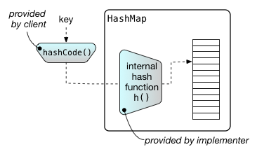
All three of these hash table implementations rely on objects
having a hashCode() method that is used to compute
the hash of an object. The hashCode() method as
defined by Java is not a hash function. As shown in the figure,
it generates the input to an internal integer hash function,
denoted as h(), which is provided by the hash table.
Therefore, the actual hash function used by the hash
table is the composition of the two methods:
h ○ hashCode.
The job of hashCode() is to hash a key object to
an int rather than to a number in
We discuss the properties of a good integer hash
function and ways to obtain it below, but now, assume that we have one.
The design of the Java collection classes is intended to relieve the client of
the burden of implementing a high-quality hash function. The use of an internal
integer hash function makes it easier to implement
hashCode() in such a way that the composed hash function
h ○ hashCode is good enough. It is easier to
implement a good hashcode than it is a good hash function.
However, a poorly designed hashCode() method can still cause the hash table
implementation to fail to work correctly or to exhibit poor performance. There are
two main considerations:
For the hash table to work, the hashCode() method must be
consistent with the equals() method, because equals()
is used by the hash table to determine when it has found the right element or key.
Otherwise the hash table might look in the wrong bucket.
In fact, it is a general class invariant of Java classes that if two objects
are equal according to equals(), then their hashCode() values
must be the same. Many classes in the Java system library do a quick check for equality
of objects by comparing their hash values and returning false if they
are not equal. If the invariant did not hold, there would be false negatives.
If you ever write a class that overrides the equals() method of Object,
be sure to do it in such a way that this invariant is maintained.
The hashCode() function should also be as injective as possible. That
is, hashing two unequal keys should be unlikely to produce the same hash code.
This goal implies that the hash
code should be computed using all of the information in the object that
determines equality. If some of the information that distinguishes two objects
does not affect the hash code, objects will always collide when they differ
only with respect to that ignored information.
Java provides a default implementation of hashCode(), which
returns the memory address of the object. For mutable objects, this implementation
satisfies the two conditions above. It is usually the right choice,
because two mutable objects are only really equal if they are
the same object. On the other hand, immutable objects such as
Strings and Integers have a notion of equality that
ignores the object's memory address, so these classes override
hashCode().
An alternative way to design a hash table is to give the job of
providing a high-quality hash function entirely to the client code:
the hash codes themselves must look random. This approach puts more
of a burden on the client but avoids wasted computation when the
client is providing a high-quality hash function already. In the
presence of keys generated by an adversary, the client should already
be providing a hash code that appears random (and ideally one with at
least 64 bits), because otherwise the adversary can engineer hash code
collisions. For example, it is possible to choose strings such that
Java's String.hashCode() produces collisions.
Immutable data abstractions such as String would normally define
their notion of equality in terms of the data they contain rather than their
memory address. The hashCode() method should therefore return
the same hashcode for objects that represent the same data value. For large
objects, it is important in general to use all of the information that makes
up the value; otherwise collisions can easily result. Fortunately, a
hash function that operates on fixed-sized blocks of information can be
used to construct a hash function that operates on an arbitrary amount of data.
Suppose the immutable object can be uniquely encoded as a finite sequence of integer
data values \(d_{1}, d_{2}, ..., d_n\), and we have an
integer hash function \(h\) that maps any integer value into a integer
hash value with good diffusion. In that case, a good hash function \(H\) can be constructed iteratively
by feeding the output of \(H\) on all previous values to \(h\).
Using \(H_{i}\) to represent the hash of the first \(i\)
values in the sequence, and ⊕ to represent the bitwise exclusive or operator, we have:
\[ H_{1} = h(d_{1}) \] \[ H_{i+1} = h(H_{i} ⊕ d_{i+1}) \] \[ H(d_{1}, ..., d_n) = H_{n} \]
Diagrammatically, the computation looks as follows:
Note that this is very different from the alternative of hashing all the individual data values and combining them with exclusive-or. That perhaps tempting algorithm would tend to have more collisions because the commutativity and associativity of exclusive-or would cause that algorithm to give the same result on any permutation of the data values.
To make hash values unpredictable across runs, it is desirable to compute the first hash value in the sequence by combining it with an initialization vector: \( H_1 = h(d_1 ⊕ IV) \), where the initialization vector \(IV\) is chosen randomly at the start of the application. It is also possible to refresh initialization vectors periodically and proactively to guard against an adversary who is trying to learn the hash function.
If writing a loop to implement the diagram above seems like too much work, a useful trick for constructing a good hashCode() method is to leverage the
fact that Java String objects implement hashCode() in this way, using
the characters of the string as the data values. If your class defines a toString()
method in such a way that it returns the same strings exactly when two objects are equal, then
hashCode() can simply return the hash of that string!
  // Requires: o1.toString().equals(o2.toString()) if and only if o1.equals(o2)
  int hashCode() {
    return toString().hashCode();
  }
One Java pitfall to watch out for arises because Java's collection classes
also override hashCode() to compute the hash from the current
contents of the collection, as if Java collections were immutable. This way of
computing the hash code is dangerous, precisely because collections are
not immutable. Mutating the collection used as the key will change
its hash code, breaking the class invariant of the hash table. Any collection
being used as a key must not be mutated.
High-quality hash functions can be expensive. If the same values are being hashed repeatedly, one trick is to precompute their hash codes and store them with the value. Hash tables can also store the full hash codes of values, which makes scanning down one bucket fast; there is no need to do a full equality test on the keys if their hash codes don't match. In fact, if the hash code is long and the hash function is cryptographically strong (e.g., 64+ bits of a properly constructed MD5 digest), two keys with the same hash code are almost certainly the same value. Your computer is then more likely to get a wrong answer from a cosmic ray hitting it than from a collision in random 64-bit data.
Precomputing and storing hash codes is an example of a space-time tradeoff, in which we speed up computation at the cost of using extra memory.
When the distribution of keys into buckets is not random, we say that the hash table exhibits clustering. If you care about performance, it's a good idea to test your hash function to make sure it does not exhibit clustering. With any hash function, it is possible to generate data that cause it to behave poorly, but a good hash function will make this unlikely.
A good way to determine whether your hash function is working well is to measure clustering. If bucket \(i\) contains \(x_i\) elements, then a good measure of clustering is the following:
A uniform hash function produces clustering \(C\) near 1.0 with high probability. A clustering measure \(C\) that is greater than one means that clustering will slow down the performance of the hash table by approximately a factor of \(C\). For example, if \(m = n\) and all elements are hashed into one bucket, the clustering measure evaluates to \(n\). If the hash function is perfect and every element lands in its own bucket, the clustering measure will be 0. If the clustering measure is less than 1.0, the hash function is spreading elements out more evenly than a random hash function would. For example, if the keys are sequential integers, and the hash function is just "mod \(m\)", the keys will be distributed as evenly as possible among the buckets, more evenly than if they were mapped randomly onto buckets. In general, you should not count on this happening!
The reason the clustering measure works is because it is based on an estimate of the variance of the distribution of bucket sizes. If clustering is occurring, some buckets will have more elements than they should, and some will have fewer. So there will be a wider range of bucket sizes than one would expect from a random hash function.
Note that it's not necessary to compute the sum of squares of all bucket lengths; picking enough buckets so that enough keys are counted (say, at least 100) is good enough.
Unfortunately, most hash table implementations, including those in the Java Collections Framework, do not give the client a way to measure clustering. Clients can't easily tell whether the hash function is performing well. We can hope that it will be standard practice for future hash table designers to provide clustering estimation as part of the interface.