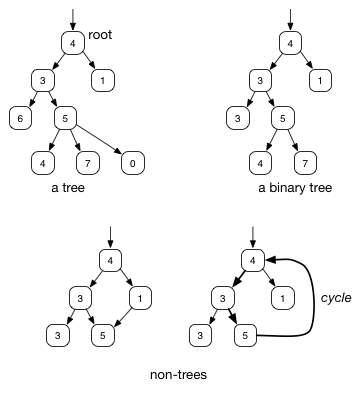
Trees are a very useful class of data structures. Like (singly-)linked lists, trees are acyclic graphs of node objects in which each node may have some attached information. Whereas linked list nodes have zero or one successor nodes, tree nodes may have more. Having multiple successor nodes (called children) makes trees more versatile as a way to represent information and often more efficient as a way to find information within the data structure.
Like lists, trees are recursive data structures. A non-empty tree has a single root node that is the starting point for searching in the tree. All nodes in the tree are reachable from the root by following a path of edges. All nodes except the root have exactly one predecessor node, called its parent. The root is the only node with no parent.
In computer science, it is customary to draw trees growing downward:
Because a tree is a recursive data structure, each node in the tree is the root of a subtree. For example, in the following tree, the node G has two children B and H, each of which is the root of a subtree. This tree is a binary tree in which each node has up to two children. We say that a binary tree has a branching factor of 2. The children of a node are usually ordered from left to right, so B is the left child of G and root of the left subtree of G, and H is the right child of G and root of the right subtree of G. A node with no children is called a leaf.
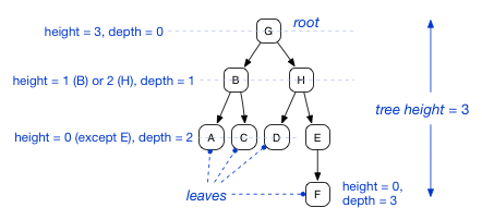
Each node in a tree has a height and a depth. The depth of a node is the length of the (unique) path from the root down to that node. The length of a path is the number of edges in the path. Thus the depth of the root is always 0. The height of a node is the length of the longest path from that node to a leaf below it. The height of the tree is the height of its root, which is the same as the depth of its deepest leaf.
We can represent a binary tree using a class with instance variables for the left and right children:
BinaryNode
For trees with a larger branching factor, the children can be stored in another data structure such as an array or linked list:
NAry
Analogously to doubly-linked lists, tree nodes in some tree data structures maintain a pointer to their parent node. A parent pointer can be useful for walking upward in a tree, though it takes up extra memory and creates additional maintenance requirements.
There are two main reasons why tree data structures are important:
Some information has a natural tree-like structure, so storing it in trees makes sense. Examples of such information include parse trees of expressions, inheritance and subtyping hierarchies, game search trees, and decision trees.
Trees make
it possible to find information within the data structure relatively quickly.
If a significant fraction of the nodes have more than one child, it can be
arranged that all nodes are fairly close to the root. For simplicity, let's
think about a complete binary tree of height h in which all leaves are at equal depth h and all non-leaves have exactly two children. In a complete binary tree of depth h, there are 1 + 2
+ 4 + ・・・ + 2h = 2h+1 − 1 nodes. Calling this number
of nodes n, we have h = log(n+1)-1, so h is O(log n). (Here log x is the
base 2 logarithm of x). Thus, if we are looking for information in a complete binary
tree, it can be reached along a path whose length is logarithmic in the total
information stored in the tree.
For large n, logarithmic time is a big speedup over the linear-time performance offered by data structures like linked lists and arrays. For example, log 1,000,000 is approximately 20, a speedup of around 50,000, and log 1,000,000,000 is about 30, a speedup of more than 30,000,000.
Of course, the preceding analysis relies on us knowing which path to take through the tree to find information. This can be arranged by organizing the tree as a binary search tree. Assume that the data stored in the nodes can be ordered according to some ordering relation. A binary search tree is a binary tree that satisfies the following data structure invariant:
| For each node n in the tree, all data stored in n's left subtree are less than the data stored at n, and all data stored in n's right subtree are greater than the data stored at n. |
|---|
Pictorially, we can visualize the tree relative to a given node as follows:

We can express this data structure invariant as a class invariant:
BST
Since the invariant is defined on a recursive type, it applies recursively throughout the tree, ensuring that data structure invariant holds for every node.
For the invariant to make sense, we must be able to
compare two elements to see which is greater (in some ordering). The
ordering is specified by the operation compareTo(). To
ensure that the type T has such an operation, we specify
in the class declaration that T extends Comparable<T>,
where Comparable<T> is the generic interface shown above.
The keyword extends signifies that T
is a subtype of Comparable<T>. Thus
T can be a class that implements the interface.
The compiler will prevent us from instantiating the class BinaryNode
on any type T that is not a declared subtype of Comparable<T>,
therefore the code of BinaryNode can assume that T
has the compareTo() method.
Consider what happens when we try to find a path down through the tree looking for an
arbitrary element x. We compare x to the root data value. If x is equal to the data value,
then we've already found it. If x is less than the data value and it's in the tree, it
must be in the left subtree, so we can walk down to the left subtree and look for
the element there. Conversely, if x is greater than the data value and it's in the tree, it
must by in the right subtree, so we should look for it there. In either case,
if the subtree where x must be is empty (null), the element must not be in the tree. This
algorithm can be expressed compactly as a (tail-)recursive method on BinaryNode:
BST
We've used Java's “ternary expression” here to make the code
more compact (and to show off another coding idiom!) The expression
b ? e1 : e2 is a
conditional expression whose value is the result of either
e1 or e2, depending on whether the boolean
expression b evaluates to true or false.
Since the method is tail-recursive, we can also write it as a loop. Here is a
version where the root of the tree is passed in explicitly as a parameter
n:
contains-loop
To add an element so we can find it later, it has to be added along the search path that will be used. To add an element, we first search for it. If found, it need not be added; if not found, it is added as a child of the leaf node reached along the search path. Again, this can be written easily as a tail-recursive method:
add
To see how this algorithm works, consider adding the element 3 to the tree
shown with the black arrows in the following diagram. We start at the root (2)
and go to the right (5) because 3 > 2. In the recursive call we then go to
the left (3 < 5) to node 4. Since 3 < 4, we try to go to the left but
observe left == null, and therefore create a left child containing 3,
shown by the gray arrow.

A map abstraction lets us associate values with keys and look up the value corresponding to a given key. This can be implemented storing both the keys and their associated values in the nodes and ordering the nodes in the tree by the keys. When the key is found, so is the associated value.
For some applications, it may be useful to allow duplicate elements. To allow equal elements to be stored in the same tree, we need to relax the BST invariant slightly. Given a node containing value x, we must know whether to go left or right to find the other occurrences of x. To build a tree where we go left, we relax the BST invariant so that the left subtree contains elements less than or equal to x, whereas the right subtree contains elements strictly greater than x.
It is possible to define search trees with more than two children per node. The higher branching factor means paths through the tree are shorter, but considerably complicates all of the algorithms involved. B-trees are an example of an N-ary search tree structure. In an N-ary search tree, each node contains up to N-1 elements e1,...,eN-1 and has up to N children c0,...,cN-1 arranged so that the subtrees of the children contain only elements between successive elements at the node. If a node has n children, the node contains n-1 elements obeying the following invariant:
To search for a given element, we do a binary search on the elements ei. If it is not found, the invariant indicates the appropriate child subtree to search.
So far we have only had pointers going downward in the tree. It is sometimes handy to have pointers going from nodes to their parents, much as nodes in a doubly linked list contain pointers to their predecessor nodes.
Removing elements from a tree is generally more complicated than adding them, because the elements to be removed are not necessarily leaves. The algorithm starts by first finding the node containing the value x to be removed and its parent node p. There are three cases to consider:
In this case, we prune the node x from the tree by setting the pointer to it from p to null. The other subtree of p (shown as a white triangle, but it may be empty) is unchanged.

We splice out node x from the tree by redirecting the pointer from p to x to now point to the single child of x. Since the BST invariant guarantees that A < x < p < B, this operation preserves the invariant.

In this case it's not as easy to remove node x. Instead, we replace the data in the node with the data from either the immediate next or the immediate previous element in the tree. Let's take the immediate next; call it x'. Since x' is the immediately next element, it must occur in the right subtree, and its node cannot possibly have a left child. Therefore, we either prune x' (if it is a leaf) or splice it out (if it is not), and then overwrite the data in node x with the data from node x'.

To find x' from x, we walk one step down the tree to the right, then walk down to the left as far as possible. The last node we encounter is x'. If x' is a leaf, we can simply remove it. If x' has a right child y, we splice x' out by making y a new child of the parent p of x'. The node y becomes the new left child of p unless p is x, in which case y becomes the new right child of x. The BST invariant is maintained!
The time required to search for elements in a search tree is in the worst case proportional to the longest path from the root of the tree to a leaf, or the height of the tree, h. Therefore, tree operations take O(h) time.
With the simple binary search tree implementation we've seen so far,
the worst performance is seen when elements are inserted in order, e.g.:
add(1), add(2), add(3), ..., add(n). The resulting binary tree
will only have right children and will be functionally identical to a linked list!

For this tree, h is O(n), and tree operations are O(n). Our goal is logarithmic performance, which requires h to be O(log n). A tree in which h is O(log n) is said to be balanced. Many techniques exist for obtaining balanced trees.
One simple-minded way to balance trees is to insert elements into the tree in a random order. This turns out to result in a tree whose expected height is O(log n) (Proving this is outside the scope of this course, but see [1, Chapter 12.4] or [2, Lecture 13] for a proof). However, we need to know how to shuffle a collection of elements into a random order, which involves a small digression:
The Fisher–Yates algorithm (developed in 1938) places N elements into random order. Recall that there are N! possible permutations of N elements; a perfectly random shuffle should have equal probability 1/N! of producing any given permutation. The algorithm works as follows. Assume we have the N elements in an array. We iterate from N–1 down to 0 deciding which element to place into a given array index. In each array index we randomly choose one of the elements in the array indices up to that point and swap it with the current array index.
fisher-yates.java
The first iteration generates one of N possible values, the second iteration one of N–1 possible values, and so on until the final iteration generates one of two possible values. Therefore, the total number of possible ways to execute is N × (N–1) × (N–2) × ・・・ × 2 = N!. Furthermore, given a particular permutation, there is exactly one way for the algorithm to produce it. Therefore, all permutations are produced with equal probability, assuming the random number generator is truly random.
Given a tree containing some number of elements, it is sometimes useful to traverse the tree, visiting each element and doing something with it, such as printing it out or adding it to another collection.
The most common traversal strategy is in-order traversal, in which each element is visited between the elements of the subtrees. In-order traverse can be expressed easily using recursion:
inorder
(Here the visit method is just some function that does something with the data.)
For example, consider using this algorithm on the following search tree:

The elements will be visited in the order 1, 3, 5, 10, 11, 17.
The traversal is not tail-recursive and therefore cannot be easily converted into a loop, but this is not a problem unless the tree is very deep. If iterative traversal is required, it can be done if nodes contain parent pointers, or with a stack to remember the nodes in the path from the root down to the node currently being visited.
Note that an in-order traversal of a binary search tree visits the elements in sorted order. This observation gives us an asymptotically efficient sorting algorithm. Given a collection of elements to sort, we first shuffle them into a random order, then add them one at a time into a BST, taking O(hn) time. Because the elements are in random order, the expected height h is O(log n), so adding all the elements takes O(n log n) time. Then we can use an in-order traversal, taking O(n) time, to extract all the elements in their proper order. While no general sorting algorithm is more efficient asymptotically than O(n log n), we will later see some other sorting algorithms that are just as asymptotically efficient but have lower constant factors.
Other traversals can be done. By visiting a node before visiting either of its children, we obtain preorder traversal. By visiting a node after visiting both of its children, we obtain postorder traversal.
pre
post
For example, a preorder traversal of the tree above would visit the nodes in the order 5, 3, 1, 11, 10, 17, and a postorder traversal would visit the nodes in the order 1, 3, 10, 17, 11, 5.