Dijkstra's single-source shortest path algorithm
Topics:
- The single-source shortest path problem
- Dijkstra's algorithm
- Proving correctness of the algorithm
- Extensions: generalizing distance
- Extensions: A*
The single-source shortest path problem
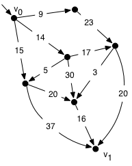
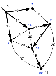
Suppose we have a weighted directed graph, and we want to find the path between two vertices with the minimum total weight. Interpreting edge weights as distances, this is a shortest-path problem. In the example illustrated, there is a path with total weight 50, but may not be easy to find it. We could find the shortest path by enumerating all possible permutations of the vertices and checking which one, but there are O(V!) such permutations.
Finding shortest paths in graphs is very useful. We have already seen an algorithm for finding shortest paths when all weights are 1, namely breadth-first search. BFS finds shortest paths from a root node or nodes to all other nodes when the distance along a path is simply the number of edges. In general it is useful to have edges with different “distances”, so shortest-path problems are expressed in terms of weighted graphs, where the weights represent distances. (Weighted undirected graphs can be regarded as weighted directed graphs with directed edges of equal weight in each direction.)
Both breadth- and depth-first search are instances of the abstract tricolor algorithm. The tricolor algorithm is nondeterministic: it allows a range of possibilities for each next step. BFS and DFS resolve the nondeterminism in different ways and visit nodes in different orders. In this lecture we will see a third instance of the tricolor algorithm due to Edsger Dijkstra, which solves the single-source shortest path problem.
For simplicity, we will assume that all edge weights are nonnegative. The Bellman-Ford algorithm is a generalization that can be used in the presence of negative weights, provided there are no negative-weight cycles. Minimum distance doesn't make sense in graphs with negative-weight cycles, because one could traverse a negative-weight cycle an arbitrary number of times, and there would be no lower bound on the weight.
We will solve the problem of finding the shortest path from a given root node or set of root nodes. If used to find a path from multiple root nodes, the algorithm will not find the distances from all of the possible starting points. To answer this question, the single-source shortest path algorithm can be used repeatedly, once for each starting node. However, if the graph is dense, it is more efficient to use an algorithm for solving the all-pairs shortest-path problem. The Floyd-Warshall algorithm is the standard algorithm, and covered in CS 3110 or CS 4820.
Dijkstra's algorithm
Dijkstra's algorithm generalizes BFS, which visits nodes in order of path length from the root. Like BFS, Dijkstra's algorithm is an instance of the tricolor algorithm. Recall that a tricolor algorithm changes nodes from white to gray and from gray to black, never allowing an edge from a black node to a white node. In Dijkstra's algorithm, the nodes are not discovered (turned from white to gray) in distance order, but they are finished (turned from gray to black) in distance order.
The progress of the algorithm is depicted by the following figure. Initially the root is gray and all other nodes are white. As the algorithm progresses, reachable white nodes turn into gray nodes and these gray nodes eventually turn into black nodes. Eventually there are no gray nodes left and the algorithm is done.
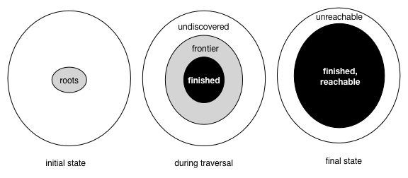
For Dijkstra's algorithm, the three colors are represented as follows:
- White nodes are undiscovered. Their distance field is set to
∞ because no path to them has been found yet. (
v.dist = ∞) - Gray nodes are frontier nodes. Their distance field is finite and is
set to the distance along some path from the root to the node. Like BFS,
the algorithm keeps track of frontier nodes in a queue, but unlike BFS,
the queue is a priority queue, which we explain shortly.
(
v.dist < ∞,v ∈ frontier) - Black nodes are finished nodes. Their distance field is set to the
true minimum distance from the root, and they are not in the priority queue.
(
v.dist < ∞,v ∉ frontier)
Dijkstra's algorithm starts with the root in the priority queue
at distance 0 (v.dist = 0), so it is gray. All other nodes are
at distance ∞ and are white. The algorithm then works roughly like BFS, except
that when node is popped from the priority queue, the node with
the smallest v.dist value among all those on
the queue is popped. When the algorithm completes,
all reachable nodes are black and hold their true minimum distance.
Here is the pseudo-code:
frontier = new PriorityQueue();
root.dist = 0;
fronter.push(root);

while (frontier not empty) {
  v = frontier.pop();  // extracts element with smallest v.dist on the queue
  foreach (Edge (v,v')) {
    if (v'.dist == ∞) {
      v'.dist = v.dist + weight(v,v');
      frontier.push(v');      // color v' gray
    } else {
      v'.dist = min(v'.dist, v.dist + weight(v,v'));
        // v' was already gray, but update to shorter distance
      frontier.adjust_priority(v');
    }
  }
  // color v black
}
Dijkstra's algorithm is an example of a greedy algorithm: an algorithm
in which simple local choices (like choosing the gray vertex with the
smallest v.dist) lead to global optimal results (minimal distances computed
to all vertices). Many other problems, such as finding a minimum spanning
tree, can be solved by greedy algorithms. Other problems cannot.
Example
Let us run the algorithm on the graph above with v0 as the root. In the first loop interation, we pop v0 and push its three successors, updating their distances accordingly. The root v0 turns black.
In the second iteration, we pop the node with the lowest distance (9) and add its successor to the queue at distance 9+23=32. The new gray frontier consists of the three nodes shown. The node at distance 9 turns black; 9 is the shortest distance to that node.
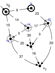
After the second iteration
The next node to come off the queue is the one at distance 14. Inspecting its successors, we discover a new white vertex and set its distance to 44=14+30. We also discover a new path of length 31=14+17 to a node already on the frontier, which is shorter than the previous best known path of length 32, so we adjust its distance.
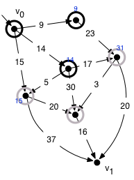
After the third iteration
We continue in this fashion until the queue becomes empty. At that point, all reachable nodes are black, and we have computed the minimum distance to each of them.
How do we recover the actual shortest paths? Observe that along any shortest path containing an edge (v,v') of weight d, v'.dist = v.dist + d. If that were not true, there would have to be another shorter path. We can't have v'.dist > v.dist+d because there is clearly a path to v' with length v.dist+d. And we can't have v'.dist < v.dist+d, because that means the original path through (v,v') was not a shortest path.
We can find the best paths by working backward from each destination vertex v', at each step finding a predecessor satisfying this equation. We iterate the process until a root node is reached. The thick edges in the previous figure show the edges that are traversed during this process. They form a spanning tree that includes every vertex in the graph and shows the minimum distance to each of them.
Performance of Dijkstra's algorithm
The algorithm does some work per vertex and some work per edge. The outer loop happens once for each vertex. The loop uses the priority queue to retrieve the vertex of minimum distance among the vertices on the queue, and there can be up to n = |V| vertices on the queue. If we implement the priority queue with a balanced binary tree, we can retrieve the minimum vertex in O(log n) time. (We cannot hope to do much better than this, otherwise we could use a priority queue to sort items faster than the known lower bound of Ω(n log n) for comparison sorting.)
We also do work proportional to the number of edges m = |E|; in the worst case every edge will cause the distance to its sink vertex to be adjusted. The priority queue needs to be informed of the new distance. This will take O(log n) time per edge if we use a balanced binary tree. So the total time taken by the algorithm is O(n log n) + O(m log n). Since the number of reachable vertices is O(m), this is O(m log n).
It turns out there is a way to implement a priority queue as a data structure called a Fibonacci heap, which makes the operation of updating the distance O(1). The total time is then O(n log n + m). However, Fibonacci heaps have poor constant factors, so they are rarely used in practice. They only make sense for very large, dense graphs where m is not O(n).
Correctness of Dijkstra's algorithm
To show this algorithm works as advertised, we will need a loop invariant.
At any stage of the algorithm, define an interior path to a node v to be a path from the root to v that goes through only black vertices, except possibly for v itself.
The loop invariant for the outer loop is then the usual tricolor black–white invariant, plus the following:
For every black vertex v and gray vertex v', v.dist ≤ v'.dist.
For every gray or black vertex, v.dist is the length of the shortest interior path to v.
-
Each iteration of the loop first colors the minimum-distance gray node v black. This preserves part 1, since the new black node was minimum over all gray nodes. Some new white successors of v will now be colored gray, but their new distances will all be greater than or equal to v.dist too. So the first part of the invariant holds. We can see from this that vertices are moved from gray to black in order of nondecreasing distance.
-
We need to show that we have the correct interior path distance to every gray or black vertex. Coloring v black doesn't create new interior paths to it, but it might create new paths to other nodes.
We don't have to worry about new interior paths to any nodes that are not successors to v, because any such interior path must have as its second-to-last step a different black node than v, one that is already at a closer distance than v. So going through v cannot produce a shorter interior path.
However, we still need to think about the interior paths to successors to v. Consider an arbitrary successor v' encountered in the inner loop. It can have one of three colors:
Black. By part 1 of the invariant, any black successor v' must have v'.dist ≤ v.dist, so there can be no shorter interior path via v.
White. By the tricolor invariant, there is no preexisting interior path to v'. Therefore the new path via v with distance v.dist+d is the only interior path.
-

Gray. If the node is already on the frontier, there is an existing interior path whose length is recorded in v'.dist. In addition, there is a new interior path to v' via v, with total distance v.dist. The code compares these two paths and picks the shorter one. Coloring v black can also create other new interior paths that don't go directly to v' via the new edge, but instead go via some other black node v''. By invariant part 1, v''.dist ≤ v.dist, so any such interior path must be at least as long as the preexisting interior path that goes from the roots directly to v'' and then to v', and we know by invariant part 2 that that path is no shorter than v'.dist.
Initialization. Part 1 of the invariant is vacuously true initially, because there are no black vertices. Part 2 is true initially, because the root is the only gray or black vertex, and root.dist is 0, which is the length of the shortest path from the root to itself.
Postcondition. When the loop finishes, all paths are interior paths, so by part 2 of the invariant, each v.dist is the length of the shortest path to v.
Preservation. Suppose the invariant holds at the beginning of the loop. We consider each of the two parts of the invariant in turn.
Generalizing shortest paths
The weights in a shortest path problem need not represent distance, of course. They could represent time, for example. They could also represent probabilities. For example, suppose that we had a state machine that transitioned to new states with some given probability on each outgoing edge. The probability of taking a particular path through the graph would then be the product of the probabilities on edges along that path. We can then answer questions such as, “What is the most likely path that the system will follow in order to arrive at a given state?” by solving a shortest path problem in a weighted graph in which the weights are the negative logarithms of the probabilities, since (−log a) + (−log b) = −log ab.
Heuristic search (A*)
Dijkstra's algorithm is a simple and efficient way to find the shortest path from a root node to all other nodes in a graph. However, if we are only interested in the shortest path to a particular vertex, it may search much more of the graph than necessary. One simple optimization is to stop the algorithm at the point when the destination vertex is popped off the priority queue. We know that v.dist is the minimal distance to v at that point because it will be colored black.
A second and more interesting optimization is to take advantage of more knowledge of distances in the graph. Dijkstra's algorithm searches outward in distance order from the source node and finds the best route to every node in the graph. In general we don't want to know every best route. For example, if we are trying to go from NYC to Mount Rushmore, we don't need to explore the streets of Miami, but that is what Dijkstra's algorithm will do.
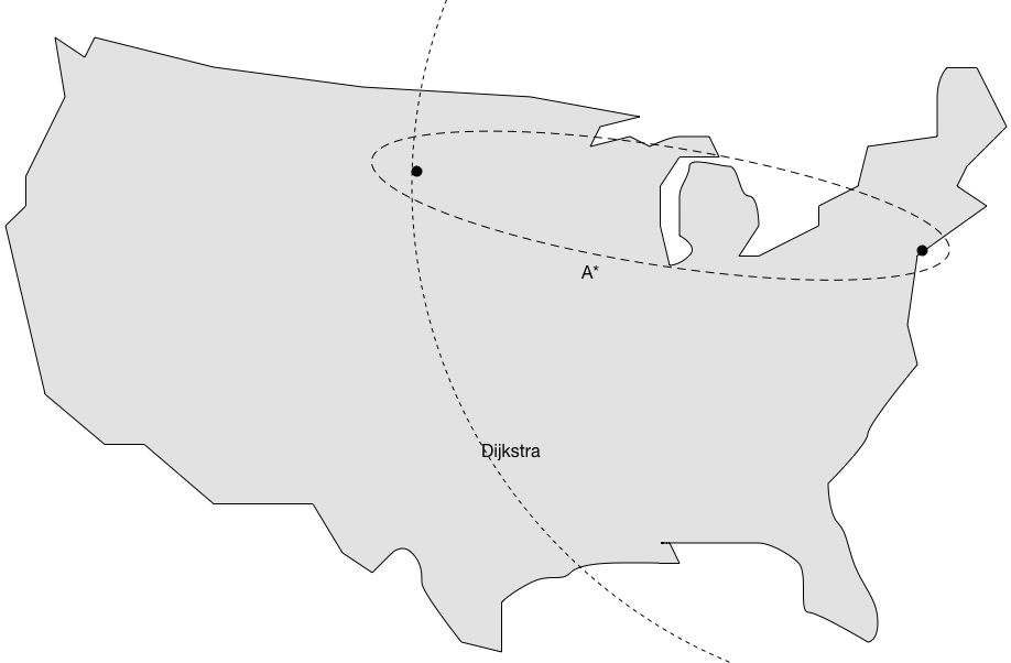
The A* search algorithm generalizes Dijkstra's algorithm to to take advantage of knowledge about the node we are trying to find. The idea is that for any given vertex, we may be able to estimate the remaining distance to the destination. We define a heuristic function h(v) that constructs this estimate. Then, the priority queue uses v.dist + h(v) as the priority instead of just v.dist. Depending on how accurate the heuristic function is, this change causes the search to focus on nodes that look like they are in the right direction.
Adding the heuristic to the node distance effectively changes the weights of edges. Given an edge from vertex v to v' with weight d, the change in priority along the edge is d + h(v') − h(v). If h(v) is a perfect estimator of remaining distance, this quantity will be zero along the optimum path; in that case we can trivially "search" for the optimum path by simply following such zero-weight edges. More realistically, h(v) will be inaccurate. If it is inaccurate by up to an amount ε, we end up searching around the optimum path in a region whose size is determined by ε.
However, we have to be careful when defining h(v). If for an edge (v,v') of weight d, the total distance including the heuristic function decreases along the edge, the conditions of Dijkstra's algorithm (nonnegative edge weights) are no longer met. In that case we have an inadmissible heuristic that could cause us to miss the optimal solution. A heuristic function is admissible if it never overestimates the true remaining distance. When searching with an admissible heuristic, each node is seen only once and the optimum path has been found immediately when the goal node is reached.
If using an inadmissible heuristic, negative-weight edges might cause us to find a new path to an already “finished” node, pushing it back on to the frontier queue. Even after finding the goal node at some distance D, It is necessary to keep searching above priority level D to account for these negative-weight edges. Despite this issue, the reason we might want to use an inadmissible heuristic is that it can be more accurate than an admissible heuristic, and thus guide the search more effectively to the goal. In some cases inadmissible heuristics can pay off.
The A* search algorithm is often used for single-player game search and various other optimization problems.