
We often want to solve problems that are expressible in terms of a traversal or search over a graph. Examples include:
The goal of a graph traversal, generally, is to find all nodes reachable from a given set of root nodes. In an undirected graph we follow all edges; in a directed graph we follow only out-edges.
Abstractly, graph traversal can be expressed in terms of the tricolor algorithm due to Dijkstra and others. In this algorithm, graph nodes are assigned one of three colors that can change over time:
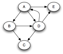
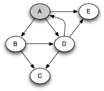
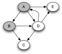
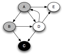
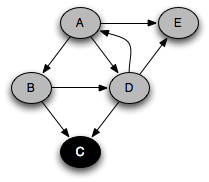
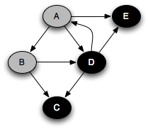
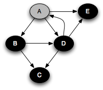
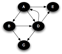
The progress of the algorithm is depicted by the following figure. Initially there are no black nodes and the roots are gray. As the algorithm progresses, white nodes turn into gray nodes and gray nodes turn into black nodes. Eventually there are no gray nodes left and the algorithm is done.
The algorithm maintains a key invariant at all times: there are no edges from white nodes to black nodes. This is clearly true initially, and because it is true at the end, we know that any remaining white nodes cannot be reached from the black nodes.
The algorithm pseudo-code is as follows:
This algorithm is abstract enough to describe many different graph traversals. It allows the particular implementation to choose the node n from among the gray nodes; it allows choosing which and how many white successors to color gray, and it allows delaying the coloring of gray nodes black. We says that such an algorithm is nondeterministic because its behavior is not fully defined. However, as long as it does some work on each gray node that it picks, any implementation that can be described in terms of this algorithm will finish. Further, because the black-white invariant is maintained, it must reach all reachable nodes in the graph.
One value of defining graph search in terms of the tricolor algorithm is that the tricolor algorithm works even when gray nodes are worked on concurrently, as long as the black-white invariant is maintained. Thinking about this invariant therefore helps us ensure that whatever graph traversal we choose will work when parallelized, which is increasingly important.
Breadth-first search (BFS) is a graph traversal algorithm that explores nodes in the order of their distance from the roots, where distance is defined as the minimum path length from a root to the node. Its pseudo-code looks like this:
// let s be the source node
frontier = new Queue()
mark root visited (set root.distance = 0)
frontier.push(root)
while frontier not empty {
    Vertex v = frontier.pop()
    for each successor v' of v {
	if v' unvisited {
	    frontier.push(v')
	    mark v' visited (v'.distance = v.distance + 1)
	}
    }
}
Here the white nodes are those not marked as visited, the gray nodes are those
marked as visited and that are in fronter, and the black nodes are
visited nodes no longer in frontier. Rather than having a visited flag,
we can keep track of a node's distance in the field v.distance. When
a new node is discovered, its distance is set to be one greater than its predecessor
v.
When frontier is a first-in, first-out (FIFO) queue, we get
breadth-first search. All the nodes on the queue have a minimum path length
within one of each other. In general, there is a set of nodes to be popped off,
at some distance k from the source, and another set of elements, later
on the queue, at distance k+1. Every time a new node is pushed onto the
queue, it is at distance k+1 until all the nodes at distance k
are gone, and k then goes up by one. Therefore newly pushed nodes are
always at a distance at least as great as any other gray node.
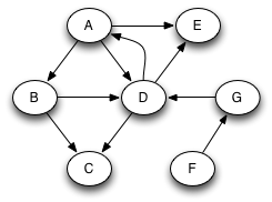
Suppose that we run this algorithm on the following graph, assuming that successors are visited in alphabetic order from any given node: :
In that case, the following sequence of nodes pass through the queue, where each node is annotated by its minimum distance from the source node A. Note that we're pushing onto the right of the queue and popping from the left.
A0 B1 D1 E1 C2
Clearly, nodes are popped in distance order: A, B, D, E, C. This is very useful when we are trying to find the shortest path through the graph to something. When a queue is used in this way, it is known as a worklist; it keeps track of work left to be done.
What if we were to replace the FIFO queue with a LIFO stack? In that case we get a completely different order of traversal. Assuming that successors are pushed onto the stack in reverse alphabetic order, the successive stack states look like this:
A
B D E
C D E
D E
E
With a stack, the search will proceed from a given node as far as it can before backtracking and considering other nodes on the stack. For example, the node E had to wait until all nodes reachable from B and D were considered. This is a depth-first search.
A more standard way of writing depth-first search is as a recursive function,
using the program stack as the stack above. We start with every node white
except the starting node and apply the function DFS to the
starting node:
DFS(Vertex v) {
    mark v visited
    set color of v to gray
    for each successor v' of v {
	if v' not yet visited {
	    DFS(v')
	}
    }
    set color of v to black
}
You can think of this as a person walking through the graph following arrows and never visiting a node twice except when backtracking, when a dead end is reached. Running this code on the graph above yields the following graph colorings in sequence, which are reminiscent of but a bit different from what we saw with the stack-based version:


Notice that at any given time there is a single path of gray nodes
leading from the starting node and leading to the current node
v. This path corresponds to the stack in the earlier
implementation, although the nodes end up being visited in a different
order because the recursive algorithm only marks one successor gray at
a time.
The sequence of calls to DFS form a tree. This is called the call tree of the program, and in fact, any program has a call tree. In this case the call tree is a subgraph of the original graph:

The algorithm maintains an amount of state that is proportional to the size of this path from the root. This makes DFS rather different from BFS, where the amount of state (the queue size) corresponds to the size of the perimeter of nodes at distance k from the starting node. In both algorithms the amount of state can be O(|V|). For DFS this happens when searching a linked list. For BFS this happens when searching a graph with a lot of branching, such as a binary tree, because there are 2k nodes at distance k from the root. On a balanced binary tree, DFS maintains state proportional to the height of the tree, or O(log |V|). Often the graphs that we want to search are more like trees than linked lists, and so DFS tends to run faster.
There can be at most |V| calls to DFS_visit. And the body of the loop on successors can be executed at most |E| times. So the asymptotic performance of DFS is O(|V| + |E|), just like for breadth-first search.
If we want to search the whole graph, then a single recursive traversal may not suffice. If we had started a traversal with node C, we would miss all the rest of the nodes in the graph. To do a depth-first search of an entire graph, we call DFS on an arbitrary unvisited node, and repeat until every node has been visited. For example, consider the original graph expanded with two new nodes F and G:
DFS starting at A will not search all the nodes. Suppose we next choose F to start from. Then we will reach all nodes. Instead of constructing just one tree that is a subgraph of the original graph, we get a forest of two trees:

One of the most useful algorithms on graphs is topological sort, in which the nodes of an acyclic graph are placed in an order consistent with the edges of the graph. This is useful when you need to order a set of elements where some elements have no ordering constraint relative to other elements.
For example, suppose you have a set of tasks to perform, but some tasks have to be done before other tasks can start. In what order should you perform the tasks? This problem can be solved by representing the tasks as node in a graph, where there is an edge from task 1 to task 2 if task 1 must be done before task 2. Then a topological sort of the graph will give an ordering in which task 1 precedes task 2. Obviously, to topologically sort a graph, it cannot have cycles. For example, if you were making lasagna, you might need to carry out tasks described by the following graph:
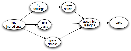
There is some flexibility about what order to do things in, but clearly we need to make the sauce before we assemble the lasagna. A topological sort will find some ordering that obeys this and the other ordering constraints. Of course, it is impossible to topologically sort a graph with a cycle in it.
The key observation is that a node finishes (is marked black) after all of its descendants have been marked black. Therefore, a node that is marked black later must come earlier when topologically sorted. A a postorder traversal generates nodes in the reverse of a topological sort:
Algorithm:
Perform a depth-first search over the entire graph, starting anew with an unvisited node if previous starting nodes did not visit every node. As each node is finished (colored black), put it on the head of an initially empty list. This clearly takes time linear in the size of the graph: O(|V| + |E|).
For example, in the traversal example above, nodes are marked black in the order C, E, D, B, A. Reversing this, we get the ordering A, B, D, E, C. This is a topological sort of the graph. Similarly, in the lasagna example, assuming that we choose successors top-down, nodes are marked black in the order bake, assemble lasagna, make sauce, fry sausage, boil pasta, grate cheese. So the reverse of this ordering gives us a recipe for successfully making lasagna, even though successful cooks are likely to do things more in parallel!
Since a node finishes after its descendents, a cycle involves a gray node pointing to one of its gray ancestors that hasn't finished yet. If one of a node's successors is gray, there must be a cycle. To detect cycles in graphs, therefore, we choose an arbitrary white node and run DFS. If that completes and there are still white nodes left over, we choose another white node arbitrarily and repeat. Eventually all nodes are colored black. If at any time we follow an edge to a gray node, there is a cycle in the graph. Therefore, cycles can be detected in O(|V+E|) time.
We can classify the various edges of the graph based on the color of the node reached when the algorithm follows the edge. Here is the expanded (A–G) graph with the edges colored to show their classification.
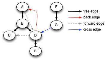
Note that the classification of edges depends on what trees are constructed, and therefore depends on what node we start from and in what order the algorithm happens to select successors to visit.
When the destination node of a followed edge is white, the algorithm performs a recursive call. These edges are called tree edges, shown as solid black arrows. The graph looks different in this picture because the nodes have been moved to make all the tree edges go downward. We have already seen that tree edges show the precise sequence of recursive calls performed during the traversal.
When the destination of the followed edge is gray, it is a back edge, shown in red. Because there is only a single path of gray nodes, a back edge is looping back to an earlier gray node, creating a cycle. A graph has a cycle if and only if it contains a back edge when traversed from some node.
When the destination of the followed edge is colored black, it is a forward edge or a cross edge. It is a cross edge if it goes between one tree and another in the forest; otherwise it is a forward edge.
It is often useful to know whether a graph has cycles. To detect whether a graph has cycles, we perform a depth-first search of the entire graph. If a back edge is found during any traversal, the graph contains a cycle. If all nodes have been visited and no back edge has been found, the graph is acyclic.
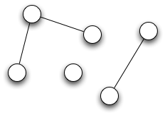
Graphs need not be connected, although we have been drawing connected graphs thus far. A graph is connected if there is a path between every two nodes. However, it is entirely possible to have a graph in which there is no path from one node to another node, even following edges backward. For connectedness, we don't care which direction the edges go in, so we might as well consider an undirected graph. A connected component is a subset S such that for every two adjacent vertices v and v', either v and v' are both in S or neither one is.
For example, the following undirected graph has three connected components:
The connected components problem is to determine how many connected components make up a graph, and to make it possible to find, for each node in the graph, which component it belongs to. This can be a useful way to solve problems. For example, suppose that different components correspond to different jobs that need to be done, and there is an edge between two components if they need to be done on the same day. Then to find out what is the maximum number of days that can be used to carry all the jobs, we need to count the components.
Algorithm:
Perform a depth-first search over the graph. As each traversal starts, create a new component. All nodes reached during the traversal belong to that component. The number of traversals done during the depth-first search is the number of components. Note that if the graph is directed, the DFS needs to follow both in- and out-edges.
For directed graphs, it is usually more useful to define strongly connected components. A strongly connected component (SCC) is a maximal subset of vertices such that every vertex in the set is reachable from every other. All cycles in a graph are part of the same strongly connected component, which means that every graph can be viewed as a DAG composed of SCCs. There is a simple and efficient algorithm due to Kosaraju that uses depth-first search twice:
For example, consider the following graph, which is clearly not a DAG:

Running a depth-first traversal in which we happen to choose children left-to-right, and extracting the nodes in reverse postorder, we obtain the ordering 1, 4, 5, 6, 2, 3, 7. Notice that the SCCs occur sequentially within this ordering. The job of the second part of the algorithm is to identify the boundaries.
In the second phase, we start with 1 and find it has no predecessors, so {1} is the first SCC. We then start with 4 and find that 5 and 6 are reachable via backward edges, so the second SCC is {4,5,6}. Starting from 2, we discover {2,3}, and the final SCC is {7}. The resulting DAG of SCCs is the following:

Notice that the SCCs are also topologically sorted by this algorithm.
One inconvenience of this algorithm is that it requires being able to walk edges backward. Tarjan's algorithm for identifying strongly connected components is only slightly more complicated, yet performs just one depth-first traversal of the graph and only in a forward direction.
See Cormen, Leiserson, and Rivest for more details.
Notes by Andrew Myers, 4/19/12.