CS 1112 Project 1 due Tue, Feb. 23, 11pm EST

Kepler’s Model of Planetary Orbits

In the 16th century, Johannes Kepler tried to explain the orbits of the then six known planets by nesting the five Platonic solids:

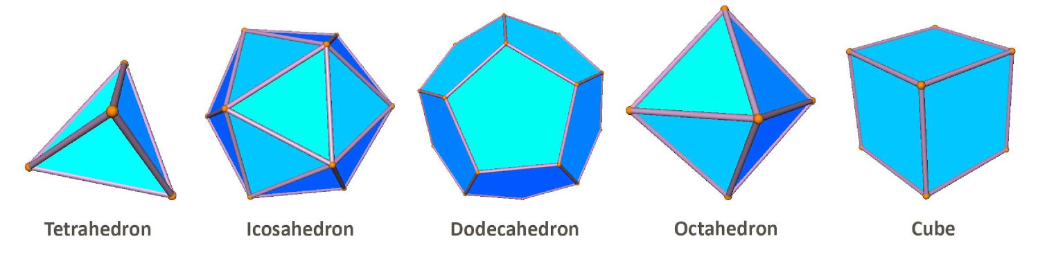
By nesting alternately a sphere and a platonic solid in a particular order, Kepler obtained sphere sizes that were proportional to the sizes of the orbits of Saturn, Jupiter, Mars, Earth, Venus, and Mercury. The nesting order of the platonic solids, from outside to inside, is the cube, tetrahedron, dodecahedron, icosahedron, and octahedron. See Kepler’s model below. Since the nesting begins with a sphere and ends with a sphere, there are six spheres with the five platonic solids in between.

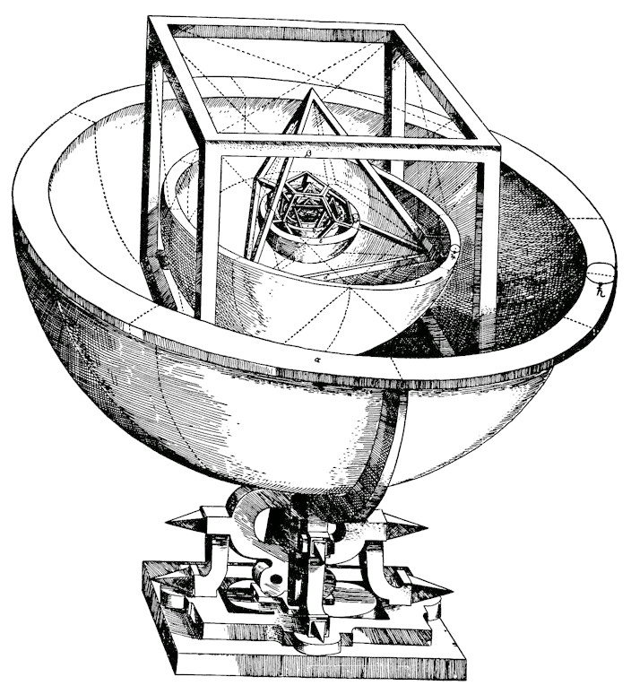
Write a script keplerModel that calculates and prints (in centimeters) the radii and circumferences of the six spheres in Kepler’s model, assuming that the outermost sphere has a radius of 1 m (we’re building a scale model), the spheres have zero thickness, and the nesting is tight. Read Problem P1.1.5 in Insight Through Computing to learn how to use the relevant formulas (but you don’t need to solve P1.1.5).

Be sure to do the calculations based on Kepler’s order for nesting the platonic solids—cube, tetrahedron, dodecahedron, icosahedron, and octahedron—not the nesting order in P1.1.5. Print the radii and circumferences neatly in a “table format,” i.e., the values should line up in columns and be printed through the 3rd decimal place. Each row of the table should include the sphere number, the radius of that sphere, and the circumference of the sphere. To do this use fprintf() with the appropriate format sequences. See, for example, scripts Eg1_2 and Eg1_1. Below, the first few lines of the “table” is shown in order to illustrate the format only—the values shown may or may not be correct.

Sphere      Radius  Circumference
     1  100.000 cm     628.319 cm
     2   57.778 cm     300.000 cm

Remember to always include units when printing dimensionful quantities, and variables storing such quantities should be commented with their units. Save your script file as keplerModel.m.

Looking through a window

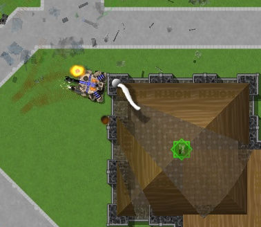
Many problems require evaluating the line-of-sight between two points (for example, illumination of solar panels, or targeting in games¹). In this exercise, you will determine whether two points can see each other through a window in a wall. You will visualize each step of the calculation graphically to check your work.

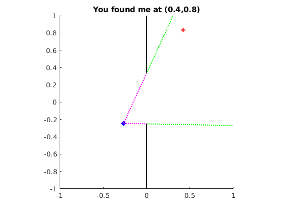
Complete the script hideAndSeek to randomly position the target, calculate the lines of sight, and produce the corresponding graphic similar to the figure above. Start by downloading the file hideAndSeek.m and running it. A figure will appear showing two black lines (the wall with a window) and a red cross (the target). The title of the plot asks you to click to the left of the wall. After you click, a blue star marks the clicked point, and its coordinates are shown in the title.

Read the program to learn what it does. Don’t worry about the early commands to set up the figure window, but here’s how the plot statement works: plot(x, y, 'r+') draws a marker at the point (x,y) with the format “red cross”; plot([x1 x2], [y1 y2], 'k-') draws a line from the point (x1,y1) to (x2,y2) with the format “black line.” Other formats are explained in the program comments. The statement [xu, yu]=ginput(1) accepts one mouse click by the user and stores the x- and y-coordinates of the click in the variables xu and yu, respectively. A statement title('hello there') would display the text “hello there” as the title of a figure. The sprintf() function works like fprintf() in formatting text, but instead of printing directly to the Command Window, sprintf() returns the text as a string to be saved under a variable name. Then this string variable can be used in other statements, such as the title statement as shown in the program.

The given program sets up a 2 × 2 “room” and demonstrates several commonly used graphics commands. You need to modify the program:

1. Change the fixed location of the target (red cross) to randomly generated coordinates within the rectangular area that is right of the wall. Hint: The statement v=rand() assigns to variable v a random number in the range of 0 to 1. Scale (multiply) and shift (add to) v as necessary to get the range you need.
2. Let the coordinates of the user-clicked point indicate the position of the seeker, which should be marked with a blue asterisk. If the user clicks to the right of the wall (ignoring instructions), change the title of the figure to “Cheater!”, and don’t perform any of the following line-of-sight calculations.
3. Start visualizing the lines-of-sight by plotting dotted lines (your choice of color) from the seeker to the top and bottom of the window.
4. Determine whether the seeker can see the target through the window. One way to do this involves logically extending the lines you just drew (but there are other methods as well). If the target can be seen, change the figure title to “You found me at (x,y)”, where x and y are the target’s coordinates (to one decimal place). If the target cannot be seen, change the title to “Still hiding”.
5. Extend the line-of-sight lines from the window to the boundary of the figure, using a different color. Stop drawing the line as soon as it reaches a boundary (either top, bottom, or right).

When developing your solution, test your changes after implementing each step before moving on to the next one.

Quadratic function

Complete exercise P1.2.8 in Chapter 1 of Insight. Save the file as myParabola.m.