stopping = -1;                                          % stopping value
prompt = ['number (' num2str(stopping) ' to stop) > ']; % input prompt
num = input(prompt);                                    % current input value
% value and frequency of leftmost mode so far of input, excluding $num$
    mode.value = NaN;
    mode.count = 0;
% value and length of "current" run, which ends on the input value before $num$
    crt.value = NaN; % or: $num$
    crt.count = 0;
% read $stopping$-terminated input sequence
% inv: maintain variable definitions above
while num ~= stopping
    % update current run
        if crt.value == num
            crt.count = crt.count + 1;
        else
            crt.value = num;
            crt.count = 1;
        end
    % update leftmost mode
        if crt.count > mode.count
            mode = crt;
        end
    % read next input
        num = input(prompt);
end

% display leftmost mode and its frequency
    disp(['Mode: ' num2str(mode.value)]);
    disp(['Count: ' num2str(mode.count)]);
And this is the output for two sample sequences,
the sample input and an empty sequence:
Here is the text of the mysqrt function:
If the first iteration is so predictable, why didn't
we initialize the variables appropriately, so that we start with the
"second" iteration? The answer is simplicity and uniformity of the
code. The initial values of the variables are chosen so as to
bootstrap the loop, without having to test for special conditions, and
without having to perform one step of the iteration outside of the
cycle body. Consider one possible alternative:
Note that the second algorithm has a subtle problem:
the algorithm will perform at least one step in the computation, even
when the tolerance is set to infinity. This is, of course, not
necessary. This is one way to avoid the unnecessary computation:
The testmysqrt script is very straightforward:
We can thus state that in general, output should be dealt with at
the highest level of the program, and not in individual functions. Of
course, if the specification of the function mandates output
(e.g. "display input and output variables"), then this provision does
not apply.
What should we do then? Well, the best solution is probably to
create a loop:
It is not strictly necessary for us to define an array of
tolerances in this case. We did it because this approach allows us to
have different tolerances for each call of the function by just
changing the values of some constants. It is always a good idea to
write the algorithm in the most general terms possible, making its
behavior contingent on the value of the predefined constants and/or
the input data.
To illustrate the slowdown due to unnecessary
output, run the two versions of the code below (ask for help on
tic and toc):
The implementation of the algorithm is quite straightforward. There
are, however, some important points to make:
First, we create the arrays that will store results at the very
beginning of the algorithm; these are the two bold lines
above. In Matlab this is not strictly necessary, because we can
extend the matrix at will. Why do we do it? Compare the execution of
two versions of this function, with, and without the bond lines
included. Use tic and toc to measure elapsed time.
Executing the line
Why does this difference arise? It is due to memory management
overhead. If Matlab must increase the size of a matrix, it will have
to allocate a new, larger, memory chunk for it to hold the result, and
then transfer the values stored into the old matrix into the new one.
Some internal bookkeeping will also be needed (so that it will
remember the new position of the matrix).
This basic strategy can be improved somewhat by trying to rezise
the current memory chunk in place (which is sometimes possible
depending on the operating system and the history of memory
allocations), or to increase memory allocation in larger chunks
(e.g. when new memory allocation is needed, allocate space for 100 new
matrix elements, not one only). No matter what improvements we use,
however, a significant overhead will be unavoidable if the size of the
matrix is extended often enough. In the example above we set a step
size to 1, and that leads to 32000 updates in the size of the x
and the y matrices.
The difference depends on how big matrices x, and y
will be. If they are relatively small, the difference is small. If the
resulting matrix is big, the overhead due to having to extend, and
possibly move, the matrix in memory can become quite significant. Even
small differences can accumulate fast if you perform an algorithm is
executed many times. Keep these thoughts in mind when you write
programs involving large volumes of data.
The second operation refers to the use of variable tmp
("temporary"). Its only role is to help avoid the repeated computation
of the same value. It saves some execution time, and (often) makes
programs more readable. Reuse computed values whenever you can!
Finally, note that by using the rem function we can
determine which values to save for return from the function. Using an
integer division we can directly compute the position where the result
should be stored. Note that there is no need to round the result of
i/skip, since mod(i, skip) == 0 implies that i is
divisible by skip. We could have used a separate counter to
rememember the value of the next index to use.
We now solve this problem using a more "matrix
oriented" approach:
Here is the testcelestial script:
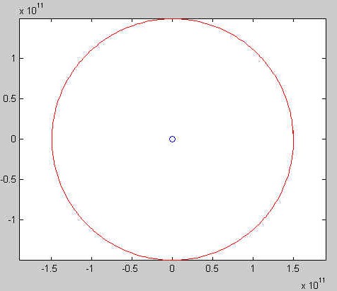
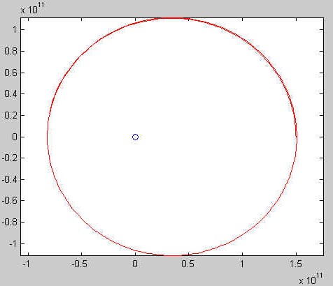
Visually, there not too much difference between the circular and
the elliptic orbit. We have used plot(0, 0, 'bo') to plot the
position of the star in these two situations. In the latter case the
star is one of the two foci of the ellipse, while in the first one it
is in the center of the circle. Experiment to find a value for
v0 that will lead to a more clearly elliptic trajectory!
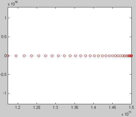
The small circles used in the case of freefall indicate the
accelerating speed of the comet. We could have used the same technique
in the other case to illustrate the changes in speed along the
trajectory. One of Kepler's laws states (qualitatively), that the
farther the comet is from the star, the slower it will move, for a
given trajectory. Can you verify this claim?
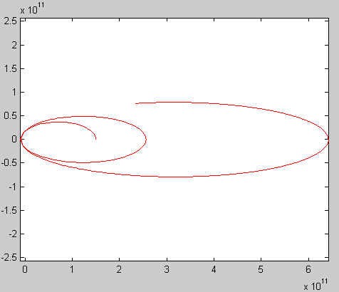
Did you notice how the trajectory of the comet gets
farther and farther away from the star? This example illustrates a
technique often employed in the space program, whereby a spaceship is
"swung" by a planet, or the Sun, often repeatedly, to gain enough
speed to reach a distant target. This allows for a lower launch speed,
and much reduced mission costs. The space ship that just landed on the
asteroid Eros swung by the Sun twice before reaching its destination.
Note the use of logical arrays to index into strings to perform
upper case conversions, and also the use of find and
num2string to generate output for an entire array in one step.
In the three solutions for T2.1 below you
should not include the bold line. Again, we show it here for the
sake of showing a specific example:
If we think a bit, we realize that we don't even need the test for
isletter. Since upper(' ') == ' ', we can just convert
to upper case all characters following a space. We don't have to make
an exception for the first character (we insert a space before it),
but we must eliminate the last one (why?). Here is this alternative
solution:
>> readmode
number (-1 to stop) > 3
number (-1 to stop) > 7
number (-1 to stop) > 8
number (-1 to stop) > 8
number (-1 to stop) > 9
number (-1 to stop) > 9
number (-1 to stop) > 9
number (-1 to stop) > 13
number (-1 to stop) > 14
number (-1 to stop) > 17
number (-1 to stop) > 17
number (-1 to stop) > 17
number (-1 to stop) > -1
Mode: 9
Count: 3
>>
>> readmode
number (-1 to stop) > -1
Mode: NaN
Count: 0
>>
Project 3: Part 2 "Give Me a Fixed Point and I Will Move the Earth..."
The implementation is quite straightforward, all we have to do is to
write a while loop to find the iteration when the change in the
computed value is less than the given precision.
function [fp, k] = mysqrt(a, epsilon)
% MYSQRT User-implemented square root.
%   [fp,k] = mysqrt(a, epsilon): compute square root $fp$ of $a$ with
%                                precision $epsilon$; $k$ is the number of
%                                iterations required

prev = -inf; % previous approximation
fp = 1;      % current approximation
k = 0;       % number of iterations performed so far

% compute successive approximations until they differ by less than $epsilson$
while abs(fp - prev) >= epsilon
    prev = fp;
    fp = (fp + a / fp) / 2;
    k = k + 1;
end
We retain two approximations of the square root, the "previous" one
prev and the "current" one fp. We also count the number
of iterations in variable k.
Note that when the while loop is first executed, the condition
is always true, except, of course, when epsilon is set to
infinite, in which case we can return any value (can you tell
why?). The first iteration only moves 1 to prev, while
computing the first "true" approximation in fp, and counting
the iteration.
% MYSQRT User-implemented square root.
%   [fp,k] = mysqrt(a, epsilon): compute square root $fp$ of $a$ with
%                                precision $epsilon$; $k$ is the number of
%                                iterations required

prev = 1;                    % previous approximation
fp = (prev + a / prev) / 2;  % current approximation
k = 1;                       % number of iterations performed so far

% compute successive approximations until they differ by less than $epsilson$
while abs(fp - prev) >= epsilon
    prev = fp;
    fp = (prev + a / prev) / 2;
    k = k + 1;
end
The computation we perform in the loop is simple in this case, so
avoiding its repetition does not lead to much saving, or improvement
in readability. For complex algorithms, however, the impact would be
much more significant.
function [fp, k] = mysqrt(a, epsilon)
% MYSQRT User-implemented square root.
%   [fp,k] = mysqrt(a, epsilon): compute square root $fp$ of $a$ with
%                                precision $epsilon$; $k$ is the number of
%                                iterations required

% compute answer for special case of $epsilon$ = $inf$
    if epsilon == inf
    	fp = 1; % any other value would do
    	k = 0;
    	return; % exit function
    end

prev = 1;                    % previous approximation
fp = (prev + a / prev) / 2;  % current approximation
k = 1;                       % number of iterations performed so far

% compute successive approximations until they differ by less than $epsilson$
while abs(fp - prev) >= epsilon
   prev = fp;
   fp = (prev + a / prev) / 2;
   k = k + 1;
end
Again, the saving of a simple iteration step might not seem as
much. But if this step were "expensive" (in time, or other consumed
resources), the additional code would be worthwhile. As mentioned
above, all these complications are solved elegantly if we think a
minute about how to bootstrap the cycle. Take a look again at the
first version of the function!
epsilon = 10^(-6);

a = 3;
[fp k] = mysqrt(a, epsilon);
fprintf(1, 'Value of parameter a is: %.6f.\n', a);
fprintf(1, 'Value of fixed point: %.8f.\n', fp);
fprintf(1, 'Number of iterations: %d.\n\n', k);

a = 4;
[fp k] = mysqrt(a, epsilon);
fprintf(1, 'Value of parameter a is: %.6f.\n', a);
fprintf(1, 'Value of fixed point: %.8f.\n', fp);
fprintf(1, 'Number of iterations: %d.\n\n', k);

a = 5;
[fp k] = mysqrt(a, epsilon);
fprintf(1, 'Value of parameter a is: %.6f.\n', a);
fprintf(1, 'Value of fixed point: %.8f.\n', fp);
fprintf(1, 'Number of iterations: %d.\n\n', k);

a = 9;
[fp k] = mysqrt(a, epsilon);
fprintf(1, 'Value of parameter a is: %.6f.\n', a);
fprintf(1, 'Value of fixed point: %.8f.\n', fp);
fprintf(1, 'Number of iterations: %d.\n\n', k);
The corresponding output is given below:
Value of parameter a is: 3.000000.
Value of fixed point: 1.73205081.
Number of iterations: 5.

Value of parameter a is: 4.000000.
Value of fixed point: 2.00000000.
Number of iterations: 5.

Value of parameter a is: 5.000000.
Value of fixed point: 2.23606798.
Number of iterations: 5.

Value of parameter a is: 9.000000.
Value of fixed point: 3.00000000.
Number of iterations: 6.
Warning: The repetition of the three fprintf statements
seems like a waste, and it is tempting to include them in the function
that performs the computation. Here is one possibility of doing it:
function [fp, k] = mysqrt(a, epsilon)
% MYSQRT User-implemented square root.
%   [fp,k] = mysqrt(a, epsilon): compute square root $fp$ of $a$ with
%                                precision $epsilon$; $k$ is the number of
%                                iterations required

prev = -inf; % previous approximation
fp = 1;      % current approximation
k = 0;       % number of iterations performed so far

% compute successive approximations until they differ by less than $epsilson$
while abs(fp - prev) >= epsilon
    prev = fp;
    fp = (fp + a / fp) / 2;
    k = k + 1;
end

fprintf(1, 'Value of parameter a is: %.6f.\n', a);
fprintf(1, 'Value of fixed point: %.8f.\n', fp);
fprintf(1, 'Number of iterations: %d.\n\n', k);
The mysqrt script is much shorter now:
epsilon = 10^(-6);

mysqrt(3, epsilon);
mysqrt(4, epsilon);
mysqrt(5, epsilon);
mysqrt(9, epsilon);
Note that we don't even need to save the values returned by the
function, all printing is done in the function's body. While "pushing"
code to the function level seems like a good idea, it most likely is
not. Good programs are written with reuse in mind, and it is
unlikely that computing a square root is a goal in itself. The users
of the mysqrt function will likely want to use the values in
more complex computations. Generating spurious output will be at least
annoying to them, but it will also slow down their program
significantly, and may destroy the structure of the text thay actually
want to display.
tolerance = 10^(-6);

a = [ 3 4 5 9];
epsilon = [tolerance tolerance tolerance tolerance];

for i = 1 : length(a)
   [fp k] = mysqrt(a(i), epsilon(i));
   fprintf(1, 'Value of parameter a is: %.6f.\n', a(i));
   fprintf(1, 'Value of fixed point: %.8f.\n', fp);
   fprintf(1, 'Number of iterations: %d.\n\n', k);
end
tic;
for i = 1:100
    disp(i);
end
toc
tic;
for i = 1:100
end
toc
Project 3: Part 3 "Celestial Bodies"
While this problem is quite complicated to state, its implementation
is relatively short. Here is one possible implementation of the
celestial function.
function [x, y] = celestial(K, dt, R0, v0, N, skip)
% CELESTIAL simulates movement under the effects of gravitation.
% see project write-up for definitions of parameters

% history of every $skip$-th position is (x, y)
    x = zeros(1, 1 + floor(N / skip));
    y = zeros(1, 1 + floor(N / skip));
% set initial position (x(1), y(1))
    x(1) = R0;
    % y(1) is already 0
% current position is (xC, yC)
    xC = R0;
    yC = 0;
% current velocity is (vxC, vyC)
    vxC = 0;
    vyC = v0;
% compute $N$ time steps
for i = 1 : N
    % compute new position (newXC, newYC)
    	newXC = xC + vxC * dt;
    	newYC = yC + vyC * dt;
    % update velocity to new velocity
    	tmp = K * dt / (xC * xC + yC * yC) ^ (3 / 2);
    	vxC = vxC - xC * tmp;
    	vyC = vyC - yC * tmp;
    % update position to new position
    	xC = newXC;
    	yC = newYC;
    % record every $skip$-th position in history
    	if rem(i, skip) == 0
    	    idx = i / skip + 1; % index of where to record current position
    	    x(idx) = xC;
    	    y(idx) = yC;
    	end
end
>> tic; [x, y] = celestial2(13.27*10^19, 1000, 1.5*10^11, 29700, 32000, 1); toc
takes 34.7600 seconds with the bold lines included, and 240.5260
seconds without them. Note that these values depend on the
computer and the operating system, so yours might be different.
function [x, y] = celestial(K, dt, R0, v0, N, skip)
% CELESTIAL simulates movement under the effects of gravitation.
% see project write-up for definitions of parameters

% history of every $skip$-th position is (x, y)
    x = zeros(1, 1 + floor(N / skip));
    y = zeros(1, 1 + floor(N / skip));
% set initial position (x(1), y(1))
    x(1) = R0;
    % y(1) is already 0
% crt = [xC yC vxC vyC]
% holds current position (xC, yC) and current velocity (vxC, vyC)
    crt = [R0 0 0 v0];
% compute $N$ time steps
for i = 1 : N
    % update current position and velocity to new position and velocity
        tmp = K * dt / sum(crt(1:2) .* crt(1:2)) ^ (3 / 2);
        crt = crt + [crt(3:4) crt(1:2)] .* [dt dt -tmp -tmp];
    % record every $skip$-th position in history
        if mod(i, skip) == 0
            idx = i / skip + 1;  % index of where to record current position
            x(idx) = crt(1);
            y(idx) = crt(2);
        end
end
Follow the code carefully to understand what it does. This
solution is not significantly faster or more readable that the first
one, but many numerical algorithms have a much simpler and more
elegant, form if written in terms of arrays and/or matrices. Due to
the advantages of vectorization this often leads to significant
speed-up of computational problems.
K = 13.27*10^19;
dt = 1000;
R0 = 1.5*10^11;

speed = [0, 29700, 25000, 43000, 10000];
steps = [3200, 32000, 32000, 32000, 128000];
format = 'o    ';

for i = 1 : length(speed)
  [x, y] = celestial(K, dt, R0, speed(i), steps(i), 100);
  figure(i);
  plot(x, y, ['r' format(i)]);
  axis tight;
  axis equal;
end
Note that we saved some typing by setting up arrays with the required
parameters, and then executing a loop where the repeated function
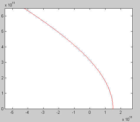
calls are executed. The five figures that we get correspond, in order,
to a free fall, a circular orbit, a (slightly) elliptic orbit, an open
(or escape, or hyperbolic) orbit, and an unstable orbit:
Project 3: Part 4 "Polynomials"
Part 4 has been moved to Project 4.
Project 3: Part 5 "Vectorization"
This is the new solution of P2.1:
% assign values to A, B
    A = [ struct('atomic_weight', 256.74, 'state', 'liquid', ...
                  'color', 'blue', 'transparency', 100), ...
          struct('atomic_weight', 107.98, 'state', 'solid', ...
                  'color', 'silver', 'transparency', 0) ];

% print A
    A(1)
    A(2)

% swap A(1), (2) - could also use A(2:-1:1), [A(2) A(1)], or fliplr(A)
    A = A([2 1]);

% print A
    A(1)
    A(2)
This our approach of solving P2.3 with
lookup tables and logical arrays. Note that the two bold lines should
not be part of your code, we included them just for the sake of taking
a specific example:
top = 'taCaGCgATAcgtg'; % input: top strand
bot = 'agTActTgATgtgC'; % input: bottom strand

% Make sure that strings are all lowercase.
    top = lower(top);
    bot = lower(bot);

% Set up the lookup table and find matching pairs.
    lookup('atgc' + 0) = 'tacg';
    match = top == lookup(bot + 0);

% Convert characters in matching positions to upper case.
    top(match) = upper(top(match));
    bot(match) = upper(bot(match));

% Show the results.
    disp(['Top sequence is:    ' top]);
    disp(['Bottom sequence is: ' bot]);
    disp(['List of matching positions: [' num2str(find(match)) '].']);
This is the associated output:
Top sequence is:    TacaGcgaTACgtG
Bottom sequence is: AgtaCttgATGtgC
List of matching positions: [1   5   9  10  11  14].
We use the lookup table to translate the top string to what its
perfectly matching complement should be. We then compare this
translation with the actual bottom string to find where they match.
str = 'cornell  has a great Computer scIence department';

idx = isspace([' ' str]) & isletter([str ' ']);
str(idx) = upper(str(idx));
We append a space to the beginning of the string so that we don't have
to treat the first character as a special case. This also serves the
useful purpose of aligning logical values that correspond to position
i-1 in the original array generated by the isspace line
up with logical values corresponding to position i generated by
the isletter function. The and operation makes sure that
only characters that are letter following a space will be converted to
upper case.
str = 'cornell  has a great Computer scIence department';

idx = find(isspace([' ' str(1:end-1)]));
str(idx) = upper(str(idx));
Now lets see how we can use findstr to solve the
same problem:
str = 'cornell  has a great Computer scIence department';

idx = findstr([' ' str(1:end-1)], ' ');
str(idx) = upper(str(idx));
Finally, here is a new solution for T1.4(a):
sides = 6;
N = 20;
D = 3;

% all $N$ outcomes; each outcome rolls $D$ dice of $sides$ sides each
    r = sum(ceil(sides * rand(D, N)));
% frequency of each *possible* outcome
    freq = hist(r, sides * D);
Each experiment is represented by the column of the random matrix that
we generate, and we have the values in these columns to obtain the
outcome of the experiment. The resulting values are stored in array
r. We then create a histogram of all the outcomes. Note that
the actual solution could have been written as a single line, with no
loss of efficiency.