MAFIA: A Maximal Frequent Itemset Algorithm For

Transactional Databases

Doug Burdick, Manuel Calimlim, Johannes Gehrke

Department of Computer Science

Cornell University

Abstract:

We present a new algorithm for mining maximal frequent itemsets from a transactional database. Our algorithm is especially efficient when the itemsets in the database are very long. The search strategy of our algorithm integrates a depth-first traversal of the itemset lattice with effective pruning mechanisms.

Our implementation of the search strategy combines a vertical bitmap representation of the database with an efficient relative bitmap compression schema. In a thorough experimental analysis of our algorithm on real data, we isolate the effect of the individual components of the algorithm. Our performance numbers show that our algorithm outperforms previous work by a factor of three to four.

1 Introduction

The association rule problem is a very important problem in the data-mining field with numerous practical applications, including consumer market-basket analysis, inferring patterns from web page access logs, and network intrusion detection [7, 16, 14]. The association rule model and the support-confidence framework were originally proposed by Agrawal et al [2, 3]. Let I be a set of items (we assume in the remainder of the paper without loss of generality I = {1, … , N}). We call a subset of I an itemset, and we call X a k-itemset if the cardinality of itemset X is k. Let database T be a multiset of subsets of I, and let support(X) be the percentage of itemsets Y in T such that X Y. Informally, the support of an itemset measures how often X occurs in the database. If support(X) > minSup, we say that X is a frequent itemset, and we write X Î FI. If X is frequent and no superset of X is frequent, we say that X is a maximally frequent itemset, and we write X Î MFI.

The process for finding association rules involves two separate phases proposed by Agrawal et al [3]. In the first phase, we find the set of frequent itemsets (FI) in the database T. In the second step, we use the set FI to generate “interesting” patterns, and various forms of interestingness have been proposed [6, 7, 9, 19, 24]. In practice, the first phase is the most time-consuming [3]. Smaller alternatives to FI in the first phase that still contain enough information for the second phase have been proposed including the set of frequent closed itemsets FCI [17, 18, 17, 27]. An itemset X is closed if there does not exist an itemset X’ such that and t(X) = t(X’), with t(Y) defined as the set of transactions that contain itemset Y. It is straightforward to see that the following relationship holds: MFI Ì FCI Ì FI.

The set MFI is orders of magnitude smaller than the set FCI, which itself is orders of magnitude smaller than the set FI. For domains where very long patterns (patterns containing many items) are present in the data, it is often impractical to generate the entire set of frequent itemsets or closed itemsets [5]. Also, there are applications where the set of maximal patterns is adequate, such as combinatorial pattern discovery in biological applications [20].

Much research has been done to develop faster methods for generating all frequent itemsets efficiently [4, 8, 10, 12, 22, 23, 25] or just the set of maximal frequent itemsets [1, 5, 11, 15, 26]. When the frequent patterns are long (more than 15 to 20 items), FI and even FCI become exponentially large and most traditional methods will end up counting too many itemsets to be feasible. Straight Apriori-based algorithms would count all of the 2^k subsets of each k-itemset they discover, and thus do not scale for long itemsets. Other methods use “lookaheads” to reduce the number of itemsets to be counted (see Section 2 for a treatment of relevant work). However, most of these algorithms use a “breadth-first” approach, i.e. finding all k-itemsets before considering (k+1) itemsets. This approach limits the effectiveness of the lookaheads, since useful longer frequent patterns have not yet been discovered. Recently, the merits of a depth-first approach have been recognized [1].

The database representation is also an important factor in the efficiency of generating and counting itemsets. Generating the itemset Z = (X Y) refers to creating t(Z) = t(X) ∩ t(Y), and counting is the process of determining support(Z) in T. Most previous algorithms use the horizontal row layout, with the database organized as a set of rows and each row representing a transaction. The alternative vertical column layout associates with each item X a set of transaction identifiers (tids) for the set t(X) [23]. The vertical representation allows simple and efficient support counting (see Section 5).

1.1 Contributions Of This Paper

In this paper, we take a systems approach to the problem of finding maximal large itemsets. We propose an efficient algorithm called MAFIA (MAximal Frequent Itemset Algorithm) that integrates a variety of old and new algorithmic contributions into a practical algorithm. MAFIA assumes that the entire database (and all data structures used for the algorithm) completely fit into main memory. With the size of current main memories reaching gigabytes and growing, many moderate-sized to large databases will soon become completely memory-resident. Considering the computational complexity involved in finding long patterns even in small databases with wide records, this assumption is not very limiting in practice. Since all algorithms for finding association rules, including algorithms that work with disk-resident databases, are CPU-bound, we believe that our study sheds light on the most important performance bottleneck.

MAFIA uses a depth-first search strategy for maximal large itemsets with pruning methods that greatly reduce the number of itemsets counted. Our implementation of MAFIA uses a vertical bitmap data layout allowing for simple, efficient itemset counting. We also describe a compression schema that reduces the size of the bitmaps and significantly increases the performance of MAFIA.

In a thorough experimental evaluation, we first quantify the effect of each individual component on the performance of the algorithm. We then compare the performance of MAFIA against DepthProject [1], the most efficient previously known algorithm for finding maximal frequent itemsets. Our results using real-life datasets indicate that MAFIA outperforms DepthProject by a factor of three to four.

1.2 Paper Organization

The organization of the paper is as follows. Section 2 discusses the conceptual ideas of the itemset lattice and subset tree we base our approach on. In Section 3, we describe the basic depth-first algorithm and methods to prune the search space. Section 4 describes the representation used for the MFI. Section 5 describes the database representation and counting methods, including compression techniques that significantly speed up the counting process. We present an analysis of the components of our algorithm and compare its performance to the DepthProject Algorithm in Section 6. We conclude in Section 7 with a discussion of future work.

2 Formulations

In this section, we describe the conceptual framework of the item subset lattice presented by Zaki in [26]. Assume there is a lexicographic ordering _Lof the items I in the database. If item i occurs before item j in the ordering, then we denote this by i_L j. This ordering can be used to enumerate the item subset lattice, or a partial ordering over the powerset S of items I. We define the partial order on S1, S2 S such that S1 S2 if S1 S2. If S1S2, there is no relationship in the ordering.

Figure 1 is a sample of a complete subset lattice for four items. The top element in the lattice is the null subset and each lower level k contains all of the k-itemsets. The k-itemsets are ordered lexicographically on each level and all children are generated from the lexicographically earliest subset in the previous level, e.g. itemset {1,2,3,4} is generated from {1,2,3}, not from itemsets {1,2,4}, {1,3,4}, or {2,3,4}. Generating children in this manner reduces the lattice to the lexicographic subset tree originally presented by Rymon [21] and adopted by both Agarwal [1] and Bayardo [5].

The itemset identifying each node will be referred to as the node’s head, while possible extensions of the node are called the tail. In a pure depth-first traversal of the tree, the tail is all items lexicographically larger than any element of the head. With a dynamic reordering scheme, the tail contains only the frequent extensions of the current node. Notice that all items that can appear in a subtree are contained in the subtree root’s head union tail (HUT), a set formed by combining all elements of the head and tail.

The problem of mining the frequent itemsets from the lattice can be viewed as finding a cut through this lattice such that all elements above the cut are frequent itemsets, and all elements (subsets) below are infrequent (see Figure 1). The frequent itemsets above the cut constitute as the positive border, while the infrequent itemsets below the cut form the negative border. With a simple traversal (i.e. no pruning), we need to count the supports of all elements above and including the negative border. For example, in Figure 1, a cut in the lattice has been drawn in and all of the itemsets shown need to be counted except for {1,2,3,4} and {1,3,4}, since they are both below the negative border.

Consider node P in Figure 1 and the cut through the lattice. P’s head is {1} and the tail (before processing) is the set {2,3,4}. Therefore, P’s HUT is {1,2,3,4}. Using dynamic reordering, P’s children {1,2}, {1,3}, {1,4} will be counted first. Based on the cut in Figure 1, only {1,2} is frequent. {3,4} will be trimmed out of the tail of P and no new itemsets need to be counted in the subtree rooted at P. In the rest of the search tree, itemsets {2,3}, {2,4}, and {3,4} would also be counted. On the other hand, a pure depth-first traversal would do extra work and compute {1,2,3}, {1,2,4}, and {2,3,4} in addition to the itemsets counted using dynamic reordering. Thus, as the size of the tree scales upward, dynamic reordering will trim out many branches of the search tree.

2.1 Related Work

Given this conceptual framework, we can describe the most recent approaches to the maximal frequent itemset problem. As a baseline, Apriori traverses the lattice in a pure breadth-first manner, discovering all frequent nodes at level k before moving to level (k+1), and only finds support information by explicitly generating and counting each node [3]. MaxMiner performs a breadth-first traversal of the search space as well, but also performs lookaheads to prune out branches of the tree [5]. The lookaheads involve superset pruning, using apriori in reverse (all subsets of a frequent itemset are also frequent). In general, lookaheads work better with a depth-first approach, but MaxMiner uses a breadth-first approach to limit the number of passes over the database.

DepthProject [1] performs a mixed depth-first traversal of the tree, along with variations of superset pruning. Instead of a pure depth-first traversal, DepthProject uses dynamic reordering of children nodes. With dynamic reordering, the size of the search space can be greatly reduced by trimming infrequent items out of each node’s tail. Also proposed in DepthProject is an improved counting method and a projection mechanism to reduce the size of the database.

The other notable maximal pattern methods are based on graph-theoretic approaches. MaxClique and MaxEclat [26] both attempt to divide the subset lattice into smaller pieces (“cliques”) and proceed to mine these in a bottom-up Apriori-fashion with a vertical data representation. However, the algorithms both rely on a pre-processing step having been performed that limits future mining flexibility. Pincer-Search [15] also assumes a pre-processing step has taken place before the algorithm executes.

The VIPER algorithm [23] has shown a method based on a vertical layout can sometimes outperform even the optimal method using a horizontal layout. It uses a vertical bitvector with compression to store intermediate data during algorithm execution, while counting is performed using a vertical tid-list approach. However, VIPER returns the entire set FI and would not be appropriate for finding the set MFI if the patterns are very long. Other vertical mining methods for finding FI are presented in [13] and [22]. An analysis of the impact of different database representations on performance can be found in [8].

3 Algorithmic Descriptions

In this section, we describe the different components of the algorithm and the various pruning methods used to reduce the search space. First, we describe the simple depth-first traversal with no pruning. We use this to motivate the pruning and ordering improvements introduced in Section 3.2.

3.1 Simple DFS

In the simple algorithm (see Figure 2), we traverse the lexicographic tree in pure depth-first order. At each node n, each element in the node’s tail is generated and counted as a possible 1-extension. If the support of {n’s head} {1-extension} is less than minSup, then we can stop by the Apriori principle, since any itemset from that possible 1-extension would have an infrequent subset. If none of the 1-extensions leads to a frequent itemset, the node is a leaf.
Algorithmic Descriptions and Pseudocode

When we reach a leaf in the tree, we have a candidate for entry into the MFI, since there are no frequent extensions of the current node. However, a frequent superset of the itemset may have already been discovered. For instance, suppose that the itemset {1,2,3,4} was already discovered to be frequent (assuming a different cut in Figure 1). When the algorithm reaches the leaf {1,2,4}, there are no frequent extensions, but a frequent superset already exists in the MFI. Therefore, we need to check if a superset of the candidate itemset is already in the MFI. If there is no superset of the candidate in the MFI, then we add the candidate itemset to the MFI. It is important to note that with the depth-first traversal, we never have to worry about removing subsets from the MFI. This is due to the fact that itemsets already inserted into the MFI will be lexicographically earlier (see Section 4 for more details on the MFI).

3.2 Pruning Away the Tree

While the simple depth-first traversal is a different exploration of the search space, it is ultimately no better than a comparable breadth-first approach, since the exact same space is generated and counted (all elements above and including the negative border). To realize performance gains, we must trim or prune out parts of the search tree by reusing information from earlier discovered frequent itemsets.

3.2.1 Parent Equivalence Pruning (PEP)

One method of pruning involves comparing the transaction sets of each parent/child pair (see Figure 3). Let x be the node n’s head and y be an element in the node n’s tail. If t(x) Í t(y), then any transaction containing x also contains y. This guarantees that any frequent itemset z containing x but not y has a frequent superset, i.e. (z È y). Since we only want the maximal frequent itemsets, it is not necessary to count itemsets containing x and not y. Therefore, we can move item y from the tail to the head. For node n, x = x y and element y is removed from n’s tail.

3.2.2 FHUT

Another type of pruning that can be used is superset pruning. We observe that at node n, the largest possible frequent itemset contained in the subtree rooted at n is n’s HUT (head union tail) as presented by Bayardo [5]. If n’s HUT is discovered to be frequent, we never have to explore any subsets of the HUT by Apriori and thus can prune out the entire subtree rooted at node n. We refer to this method of pruning as FHUT (Frequent Head Union Tail) pruning.

FHUT can be computed by exploring the leftmost path in the subtree rooted at each node. In fact, since the depth-first algorithm already explores the leftmost path, no extra computation is necessary. Careful use of passed boolean variables can determine which subtrees to prune out of the search space (see Figure 4). A disadvantage of FHUT is that the leftmost path contains the most items of any path in the subtree. Thus, while the subtree rooted at that node is pruned, a large portion of the tree is still generated and counted.

3.2.3 HUTMFI

There are two methods for determining whether an itemset x is frequent: direct counting of the support of x, and checking if a superset of x has already been declared frequent. FHUT is one method for discovering if a node’s HUT is frequent by counting the actual support of the HUT. Another way to determine HUT frequency is to check if a superset of the HUT is in the MFI. If a superset does exist, then the HUT must be frequent and the subtree rooted at that node can be pruned away. However, if no superset is found, that does not mean that the HUT is infrequent. The subtree at that node must still be explored.

We call this type of superset pruning HUTMFI (see Figure 5). Note that HUTMFI does not expand any children to check for successful superset pruning, unlike FHUT where the leftmost branch of the subtree is explored. Therefore, in general, HUTMFI is preferable to FHUT pruning.

3.3 Dynamic Reordering in MAFIA

The benefits of dynamically reordering the children of each node based on support are significant. However, dynamic reordering requires counting the support of all the extensions of a node before processing the first child and thus, would not be a pure depth-first traversal of the space.

Note that most of the elements of a node’s tail will not be frequent extensions, and since tails are formed from all elements lexicographically later than the head, these same infrequent items will appear in many tails. Therefore, an algorithm that trims the tail to only frequent extensions at a higher level will save a great deal of computation. For example in Figure 1, if the itemset {1,4} is counted and found to be infrequent, then item 4 can be trimmed from the tail of all nodes in that subtree. The end result is that the itemsets {1,2,4}, {1,3,4} need never be counted in that subtree.

The order of the children is also an important consideration. Ordering them by increasing support will keep the search space as small as possible; the less frequent nodes will have small subtrees while the more frequent nodes will appear at the end of the tail and thus will be more likely to be trimmed by superset pruning (both FHUT and HUTMFI). This heuristic was first used by Bayardo [5]. Of particular note, PEP can be applied much faster. Since PEP depends on the support of each child relative to the parent’s support, pre-counting all children can quickly identify when PEP holds. We can move all elements for which PEP holds from the node’s tail to the node’s head at once, significantly reducing the size of the tail.

Therefore, all of the components of the algorithm fit together very nicely and help trim the search space. However, certain components are more effective than others. The interaction of the different pruning mechanisms and the effect on performance is analyzed in Section 6.1.

4 Calculating Maximal Frequent Itemsets

With a depth-first traversal, all frequent itemsets found will be in lexicographic order. When a leaf is found, it is a candidate itemset, since there are no frequent extensions. These two facts have useful benefits in representing the set of Maximal Frequent Itemsets (MFI). Since elements are added to the MFI only when no frequent extensions exist and in lexicographic order, we can guarantee that no superset of the candidate itemset will be added to the MFI later in the search space. The remaining problem is determining whether a superset of the candidate itemset was added before the current itemset.

4.1 MFI Representation And Checking

Itemsets in the MFI are stored as horizontal bitmaps. Contained in the bitmap is a bit for every item in the database, e.g. the itemset {1,3,4} would be represented as the bitmap (1011). We call these bitmaps name bitmaps to distinguish them from the transaction bitmaps used for counting (see Section 5).

The name bitmaps provide a simple and efficient method for superset checking. To determine if itemset x1 is a superset of itemset x2, our algorithm will bitwise-AND the bitmaps of x1 and x2 together. If the resulting bitmap matches x2, then x2 is a subset of x1. A simple algorithm, then, for finding supersets in the MFI is to bitwise-AND the candidate itemset’s name bitmap with each element of the existing MFI. If a superset is found, the candidate itemset is not added to the MFI.

4.2 Optimization Of MFI Checks

The naïve approach to MFI checks is to search the entire MFI set for each new itemset to insert. However, this is clearly a quadratic time algorithm. As the number of items scales up and the size of the MFI grows, MFI checks can significantly slow the running time. Is there a better solution using MFI checks? An empirical analysis of the MFI checks revealed a very interesting trend: over 90% of the supersets in the MFI are found in the last 10 itemsets most recently inserted.

Therefore, a good approximation is to fix the number of itemsets checked to a constant value. The experimental data indicates that 50 itemsets yields a good compromise between accuracy and time. Stopping the search and declaring that no superset exists in the MFI can save a great deal of computation. The modification to the algorithm is simple: for each new itemset, the last 50 itemsets inserted into the MFI are checked for a possible superset. If all 50 MFI checks fail, then the new itemset is added to the MFI.

4.3 Post-Processing

While the approximation of the last K-itemsets yields dramatic savings, it also produces an MFI that is possibly slightly inaccurate. It is unlikely, but not impossible that there are supersets beyond the last 50 itemsets. Therefore, the MFI will contain extra itemsets that are subsets of maximal frequent itemsets. If an exact representation of the MFI is required, the non-maximal itemsets must be removed. Since this step would be conducted after the tree has been explored, we call it the post-pruning phase. Other maximal frequent itemset algorithms also return a superset of the MFI (MaxEclat and MaxClique [26]) and a similar post-pruning step is used by Agarwal et al. in DepthProject[1].

5 Representation of the Database

5.1 Representation

We chose to use a vertical bitmap representation for each of the items. In a vertical bitmap, there is one bit for each transaction in the database. If item i appears in transaction j, then bit j of the bitmap for item i is set to one; otherwise, the bit is set to zero. This naturally extends to itemsets. Define X as the itemset corresponding to the head of the node. Let onecount(X) be the number of ones in the vertical bitmap for X. Note that the count of ones is exactly the support of itemset X. Let bitmap(X) correspond to the vertical bitmap that represents the transaction set for the itemset X. For each element Y in the node’s tail, t(X) ∩ t(Y) is simply computed as the bitwise-AND of bitmap(X) and bitmap(Y).

5.2 Counting Support

As the fundamental step in generating each new node in the lexicographic tree, support counting must be highly optimized. This necessity motivated the vertical bitmap representation. We adapted a two-phase byte counting method for generating and counting the extensions to an itemset. Offline, we compute and store the number of 1’s a particular byte value has for all 256 possible byte values, e.g. byte value “2” has 1 one, “3” has 2 ones, and “255” has 8 ones. Generation of new itemset bitmaps involves bitwise-ANDing bitmap(X) with a bitmap for 1-itemset Y and storing the result in bitmap (X È Y). Next, for each byte in bitmap (X È Y), we lookup the number of 1’s in the byte using the pre-computed table. Summing these lookups gives the support of (X È Y).

5.3 Compression And Projected Bitmaps

The weakness of a vertical representation is the sparseness of the bitmaps, especially at the lower support levels. Since every transaction has a bit in vertical bitmaps, there are many zeros since both the absence and presence of the itemset in a transaction need to be represented. However, in some cases this is the smallest representation of the information we need possible[1]. Given the generating and counting method presented above, this presents a source of inefficiency since we are performing wasted operations over regions containing useless information (regions of only 0’s in X’s bit vector).

We can make the observation that we only need information about transactions containing the itemset X to count the support of the subtree rooted at node N. If transaction T does not contain the itemset X (X’s bit vector has a 0 in bit T), then it will not provide useful information for counting supports of N’s children and can be ignored in all subsequent operations. So, conceptually we can remove the bit for transaction T from X and all items in N’s tail. This is a form of compression of the vertical bitmaps to speed up calculations. The pseudocode describing the process can be found in Figure 7.

In the projected bit vector for X all positions have value 1, since each position corresponds to a transaction needed for computation in the subtree rooted at node N. We are guaranteed to consider every element in N’s tail at least once when traversing the subtree rooted at N. The projection operation is performed when the support of itemset X drops below a certain rebuilding_threshold, expressed as a percentage of bitmap X’s overall size (in bits).

However, there is a tradeoff on the value selected for rebuilding_threshold. As the rebuilding_threshold decreases, the cost of projection rises, since many more nodes at the lower levels of the tree will need to be projected. On the other hand, the size of the projected bitmaps is guaranteed to be smaller and thus the cost of subsequent generation and counting in that subtree is significantly reduced. In practice, we found that there is only a small difference in choosing a value for rebuilding_threshold between 0.25 and 1. Below 0.25, the cost of rebuilding exceeds the savings of using projected bitmaps, but between .25 and 1, the cost of projection is balanced by the smaller vertical bitmaps. The reason for this result is that the size of the projected bitmaps when built immediately (rebuilding_threshold = 1) depends only on the support of the frequent 1-itemsets they are projected against. In the real datasets considered, many 1-itemsets have low supports, and thus, any rebuilding_threshold above the supports will yield the same projected bitmaps.

6 Experimental Results

The experiments were conducted on a 933 Mhz Pentium III with 512 MB of memory running Microsoft Windows 2000. All code was compiled using Microsoft Visual C++ 6.0. MAFIA was tested on three datasets that have been shown to generate long patterns [1,5]: connect-4, mushroom, and chess. In general, at the higher supports, the patterns vary between 5-12 items long, while at lower supports the patterns contain over 20 items. A detailed comparison of MAFIA on these datasets was conducted, since MAFIA yields the greatest gains when mining long patterns from a database.

6.1 Algorithmic Component Analysis

First however, we present a full analysis of each component of the MAFIA algorithm (see Section 3 for algorithmic details). There are three types of pruning used to trim the tree: FHUT, HUTMFI, and PEP. FHUT and HUTMFI are both forms of superset pruning and thus will tend to “overlap” in their efficacy for reducing the search space. In addition, dynamic reordering will significantly reduce the size of the search space by removing infrequent items from each node’s tail.

Figures 9 and 10 show the effects of each component of the MAFIA algorithm on the mushroom dataset at 1% minimum support. The number of transactions was increased by repeating all transactions in the database by a certain scaling factor. We call this form of scaling vertical scaling. In this case, mushroom was scaled ten times vertically. Note that vertical scaling will not change the search space, and will only affect the time taken for counting the support of itemsets.

The components of the algorithm are represented in a cube format, where the running times for all possible combinations are shown. The top of the cube shows the time for a simple traversal where the full search space is explored, while the bottom of the cube corresponds to all three pruning methods being used. Two separate cubes (with and without dynamic reordering) rather than one giant cube are presented for readability.

Note that all pruning components yield some savings in running time, but that certain components are more effective than others. In particular, HUTMFI and FHUT yield very similar results, since they use the same type of superset pruning, but with different methods of implementation. The efficient MFI lookups that HUTMFI uses to check for frequency explains why HUTMFI outperforms FHUT (see Sections 3 and 4). It is also interesting to see that adding FHUT when HUTMFI is already performed yields very little savings, i.e. from [HM] to [HM+FH] or from [HM+PEP] to [ALL], the running times do not significantly change. HUTMFI checks for the frequency of a node’s HUT by looking for a frequent superset in the MFI, while FHUT will explore the leftmost branch of the subtree rooted at that node. Apparently, there are very few cases where a superset of a node’s HUT is not in the MFI, but the HUT is frequent.

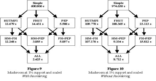
PEP has the biggest effect of the three pruning methods. All of the running time of the algorithm occurs at the lower levels of the tree where the border between frequent and infrequent itemsets exists, and since PEP is most likely to trim out large sections at the lower levels, this pruning yields the greatest results. Dynamically reordering the tail also has dramatic savings (cf. Figure 9 with Figure 10). It is interesting to note that without PEP, dynamic reordering runs nearly an order of magnitude faster than the static ordering, while with PEP, it is “only” 3-5 times faster. Since both PEP and reordering remove elements from a node’s tail, it is not surprising that they overlap in their efficacy.

6.2 Comparison With DepthProject

We tested the algorithm on “real” datasets containing long patterns that have been used earlier [1,5]. These datasets are publicly available from the UCI Machine Learning Repository. At the lowest supports tested, the longest patterns in these databases have over 20 items, making any algorithm that examines all possible subsets of these patterns (or a significant portion) infeasible. This makes the task of finding the patterns computationally intensive despite the small size of the databases. For some of the experiments the databases were scaled vertically by concatenating copies of the database together. This only affects the time counting takes since the bitmaps (compressed or not) are longer and the search space examined remains constant.

Figures 11 – 13 illustrate the results of comparing MAFIA to our implementation of the DepthProject [1] method, the state-of-the-art method for finding maximal patterns. The x-axis is the user-specified minimum support, while the Y-axis uses a logarithmic scale to show the running time.

In Figures 11 and 12, we see MAFIA is approximately four to five times faster than DepthProject on both the Connect-4 and Mushroom datasets for all support levels tested (down to 10% support in Connect-4 and 0.1% in Mushroom). These were the most striking performance improvements. For Connect-4, the increased efficiency of itemset generation and support counting in MAFIA versus DepthProject explains the improvement. Connect-4 contains an order of magnitude more transactions than the other two datasets (67,557 transactions), amplifying the MAFIA advantage in generation and counting.

For Mushroom, the improvement is best explained by how often parent-equivalence pruning (PEP) holds, especially for the lowest supports tested. While there is a large number of frequent 1-itemsets at the lowest support (115 items at 0.1% support), many items with low support can be pruned using PEP (see Section 3.2.1). When this condition holds, several items can be removed from the tail at once, saving the exploration of branches guaranteed to contain non-maximal patterns. The dramatic effect PEP has on reducing the number of itemsets generated and counted is shown in Table 1. The entries in the table are the reduction factors due to PEP (in the presence of all other pruning methods) for the first eight levels of the tree. Reduction factor is defined as (# itemsets counted at depth k without PEP) / (# itemsets counted at depth k with PEP). In the first four levels, Mushroom has the greatest reduction in number of itemsets generated and counted. This leads to a much greater reduction in the overall search space than for the other datasets, since the reduction is so great at highest levels of the tree.

Figure 11

Figure 12

Figure 14

Figure 13

Depth	1	2	3	4	5	6	7	8
Connect-4	1.23	4.22	16.46	61.07	134.8	169.06	79.98	50.43
Mushroom	1	12.64	51.81	73.15	72.92	56.81	41.29	26.78
Chess	1.33	4.14	5.73	6.51	6.73	6.7	5.97	4.95

Table 1 – Reduction Factor of Nodes Considered due to PEP pruning

In Figure 13, we see that MAFIA is only a factor of two better than DepthProject on the dataset Chess. The extremely low number of transactions in Chess (3196 transactions) and the small number of frequent 1-items at low supports (only 54 at lowest tested support) muted the factors that MAFIA relies on to improve over DepthProject. Table 1 shows the reduction in itemsets using PEP for Chess was an order of magnitude lower compared to the other two data sets for all depths.

To test the counting conjecture, we ran an experiment that vertically scaled the Chess dataset and fixed the support at 50%. This keeps the search space constant while varying only the generation and counting efficiency differences between MAFIA and DepthProject. The result is shown in Figure 14. We notice both algorithms scale linearly with the database size, but the scaleup factor for MAFIA is much smaller than for DepthProject. Similar results were found for the other datasets as well. Thus, we see MAFIA scales very well vertically.

6.3 Effects Of Compression

To isolate the effect of the compression schema on performance, experiments with varying rebuilding_threshold values were conducted. The most interesting result is on a scaled version of Connect-4, displayed in Figure 15. The connect-4 dataset was scaled vertically three times, so the total number of transactions is approximately 200,000. Three different values for rebuilding_threshold were used: 0 (corresponding to no compression), 1 (compression immediately, and all subsequent operations performed on compressed bitmaps), and an optimized value tied to minSup (the greater of (2* minSup) or 25%). We see for higher supports above 40% compression has a negligible effect over no compression, but at the lowest supports compression can be quite beneficial, e.g. at 10% support compression yields a savings factor of 3.6.

However, the small difference between compressing immediately and finding an optimal compression point is not so easily explained. The greatest savings here is only 11% at the lowest support of Conenct-4 tested. Another experiment where support was fixed and the Connect-4 dataset was scaled vertically was performed to isolate the effect of the different rel_threshold values. The results appear in Figure 16. The x-axis shows the scale up factor while the y-axis displays the running times. We can see that the optimal compression scales the best. For many transactions (over 10⁶), the optimal rel_threshold outperforms compressing everywhere by approximately 35%. In any case, both forms of compression scale much better than no compression.

Figure 15

Figure 16

6.4 Raw Data Gathered During Experiments

Included in these tables are the number of maximal frequent itemsets, the number of itemsets found by MAFIA, and the comparative running times (in seconds) of MAFIA and DepthProject at various supports.

Connect-4
% support	90	80	70	60	50	40	30	20	10
MFISize	222	673	1220	2103	3758	6213	11039	32571	130986
Itemsets found	222	673	1220	2103	3758	6213	11039	32571	130986
MAFIA	0.11	0.36	0.72	1.28	2.34	2.72	4.19	9.45	35.12
DepthProject	0.23	1.16	3.20	5.70	10.03	16.51	26.26	50.77	134.90

Table 2

Mushroom
% support	10	7.5	5	2.5	1	0.1
MFISize	547	909	1442	3036	6768	27712
Itemsets found	629	1046	1789	3969	8946	36873
MAFIA	0.07	0.08	0.14	0.25	0.46	1.08
DepthProject	0.18	0.23	0.80	0.87	1.77	5.92

Table 3

Chess
% support	60	55	50	45	40	35	30	25	20
MFISize	3323	6262	11463	20628	38050	71166	134624	260092	509335
Itemsets Found	3330	6318	11693	21280	39813	75838	146655	290774	588858
MAFIA	0.14	0.25	0.48	0.70	1.22	2.20	3.75	6.98	13.8
DepthProject	0.25	0.45	0.76	1.29	2.26	4.12	7.88	14.72	28.66

Table 4

7 Conclusions

In this paper we presented MAFIA, an algorithm for finding maximal frequent itemsets, which uses a depth-first traversal of the search space. Our experimental results demonstrated MAFIA consistently outperformed DepthProject, which represents the state-of-the-art in finding maximal frequent itemsets in data with large itemsets, by a factor of 3 to 4. The breakdown of the algorithmic components showed parent-equivalence pruning and dynamic reordering were quite beneficial in reducing the search space while relative compression/projection of the vertical bitmaps dramatically cuts the cost of counting supports of itemsets and increases the vertical scalability of MAFIA.

For future work, we propose exploring application of the depth-first search with vertical bitmap representation to find the set of frequent closed itemsets (FCI). Also, modifications of the algorithm to handle disk-resident data and to use more advanced compression techniques for the bitmaps will be pursued.

8 Acknowledgements

We would like to thank Charu Aggarwal for discussing DepthProject and giving us advise on its implementation. We also thank Jayant R. Haritsa for his insightful comments on the MAFIA algorithm and Jiawei Han for helping in our understanding of CLOSET and providing us the executable of the FP-Tree algorithm.

References:

[1] R. Agarwal, C.Aggarwal, and V. V. V. Prasad. A Tree Projection Algorithm for Generation of Frequent Itemsets. In Journal of Parallel and Distributed Computing (special issue on high performance data mining), (to appear), 2000.

[2] R. Agrawal, T. Imielinski, and R. Srikant. Mining association rules between sets of items in large databases. SIGMOD, May 1993.

[3] R. Agrawal, R. Srikant: Fast Algorithms for Mining Association Rules, Proc. of the 20th Int'l Conference on Very Large Databases, Santiago, Chile, Sept. 1994.

[4] R. Agrawal, H. Mannila, R. Srikant, H. Toivonen and A. I. Verkamo, Fast Discovery of Association Rules, Advances in Knowledge Discovery and Data Mining, Chapter 12, AAAI/MIT Press, 1995.

[5] R. J. Bayardo. Efficiently mining long patterns from databases. In Proc. 1998 ACM-SIGMOD Int. Conf. Management of Data (SIGMOD ‘98), pages 85-93, Seattle, Washington, June 1998

[6] R. J. Bayardo Jr. and R. Agrawal. Mining the Most Interesting Rules. In Proc. of the 5th ACM SIGKDD Int'l Conf. on Knowledge Discovery and Data Mining, 145-154, August 1999.

[7] Sergey Brin, Rajeev Motwani, Jeffrey D. Ullman, and Shalom Tsur. Dynamic itemset counting and implication rules for market basket data. SIGMOD Record (ACM Special Interest Group on Management of Data), 26(2):255, 1997.

[8] B. Dunkel and N. Soparkar. Data Organization and access for efficient data mining. In Proc. Of 15^th Intl. Conf. On Data Engineering (ICDE), 1999.

[9] T. Fukuda, Y. Morimoto, S. Morishita, and T. Tokuyama. Data mining using two-dimensional optimized association rules: Scheme, algorithms, and visualization. In Proc. 1996 ACM-SIGMOD Int. Conf. Management of Data, pages 13--23, Montreal, Canada, June 1996.

[10] G. Gardarin, P. Pucheral, and F. Wu. Bitmap based algorithms for mining association rules. Technical report 1998-18, University of Versailles, 1998.

[11] Dimitrios Gunopulos, Heikki Mannila, Sanjeev Saluja: Discovering All Most Specific Sentences by Randomized Algorithms. ICDT 1997: 215-229

[12] Jiawei Han, Jian Pei, Yiwen Yin: Mining Frequent Patterns without Candidate Generation. SIGMOD Conference 2000: 1-12.

[13] Marcel Holsheimer, Martin L. Kersten, Heikki Mannila, Hannu Toivonen: A Perspective on Databases and Data Mining. KDD 1995: 150-155.

[14] W. Lee and S. J. Stolfo. Data mining approaches for intrusion detection. In Proceedings of the 7th USENIX Security Symposium, 1998.

[15] D.I. Lin and Z. M. Kedem. Pincer search: A new algorithm for discovering the maximum frequent sets. In Proc. of the 6th Int'l Conference on Extending Database Technology (EDBT), Valencia, Spain, 1998.

[16] B. Mobasher, N. Jain, E.H. Han, and J. Srivastava. Web mining: Pattern discovery from world wide web transactions. Technical Report TR-96050, Department of Computer Science, University of Minnesota, Minneapolis, 1996

[17] N. Pasquier, Y. Bastide, R. Taouil, and L. Lakhal. Discovering frequent closed itemsets for association rules. In Proc. 7^th Int. Conf. Database Theory (ICDT ‘99), pages 398-416, Jerusalem, Israel, January 1999.

[18] J. Pei, J. Han, and R. Mao. CLOSET: An efficient algorithm for mining frequent closed itemsets, In Proc. ACM SIGMOD Workshop on Research Issues in Data Mining and Knowledge Discovery, Dallas, TX, May, 2000.

[19] Rastogi R., and Shim K. Mining Optimized Association Rules with Categorical and Numeric Attributes. In Proceedings of the International Conference on Data Engineering, Orlando, Florida, February 1998.

[20] Rigoutsos, I., and Floratos, A. Combinatorial pattern discovery in biological sequences: The Teiresias algorithm. Bioinformatics 14, 1 (1998), 55-67.

[21] Rymon, R. 1992. Search through Systematic Set Enumeration. In Proc. Of Third Int’l Conf. On Principles of Knowledge Representation and Reasoning, 539 –550.

[22] A. Savasere, E. Omiecinski, and S. Navathe. An efficient algorithm for mining association rules in large databases. In 21st VLDB Conference, 1995.

[23] Pradeep Shenoy, Jayant R. Haritsa, S. Sudarshan, Gaurav Bhalotia, Mayank Bawa, Devavrat Shah: Turbo-charging Vertical Mining of Large Databases. SIGMOD Conference 2000: 22-33

[24] Geoffrey I. Webb. OPUS: An efficient admissible algorithm for unordered search. Journal of Artificial Intelligence Research, 3:45--83, 1996.

[25] L. Yip, K.K. Loo, Ben Kao, David Cheung, C.K. Cheng, Lgen. A Lattice-Based Candidate Set Generation Algorithm for I/O Efficient Association Rule Mining, in the Third Pacific-Asia Conference on Knowledge Discovery and Data Mining (PAKDD '99), Beijing, 1999.

[26] Mohammed J. Zaki, Scalable Algorithms for Association Mining, in IEEE Transactions on Knowledge and Data Engineering, Vol. 12, No. 3, pp 372-390, May/June 2000.

[27] M. J. Zaki and C. Hsiao. CHARM: An efficient algorithm for closed association rule mining. In Technical Report

[1] An alternative representation would be a vertical tid-list for each item, where each item has the list of transactions it appears in associated with it. Even though only the presence of items is represented, it is guaranteed to be more expensive representation in terms of space if the support of an item is greater than (1/32) or about 3%. In a vertical tid-list representation, we need an entire word (32 bits in most architectures) to represent the presence of an item versus the single bit of the vertical bitvector approach. Thus, if the item appears in more than (1/32) of the transactions, this is a less efficient representation. All methods to make this smaller involve CPU-computation (e.g. compression).