General Concepts
Solving a Problem
When solving a problem we have to create a model of the problem in which it can be solved. It is very common that we will not try to generate a solution to the real problem as is. In fact, what we commonly do is to generate a model that is an abstraction of the real problem and we try to give solutions to it. For example, when we think about the Newton's Laws of Motion we have to know that they work with a lot of assumptions and that they are really based on a model instead of the reality. Before we attempt to build a solution to a given problem we have to understand the concepts related to it, create the appropriated model and use the available tools to try to solve it.
As Michalewicz and Fogel say in their book about heuristics, a model needs a representation, an objective and also an evaluation function. That way you can know how to encode the solutions of the problem, which is the purpose of the problem and a way to evaluate if a given solution is good or not. When dealing with a problem, it is important to understand those concepts well in order to understand the problem and solve it. For example, in SAT (a problem that will be explained later) a way to represent the solutions is with a binary number where each digit represents the value of a given variable of the problem, the objective is to find an assignment that satisfies all the clauses of the problem and the evaluation function is precisely the formula where you can substitute the solution and see if it gives true as an output.
During the last six months, the research internship time, I was working with the SAT, MINSAT and QBF problems and worked on the development of an incomplete QBF solver that showed to outperform some of the best state of the art QBF solvers. Below I will talk about some basic concepts that someone new to this research area has to know to understand the SAT problem and to generate some new solutions to it.
Search Heuristics
Each problem can be solved with a different approach. Many of them are problems where you have to search for the solution on a given search space and many times those search spaces are huge and have different characteristics from one problem to other.
When searching for a solution, several approaches can be used. The two main approaches are searching with complete solutions and searching with partial solutions. When using complete solutions we can stop at any time and give to the problem a solution that may not be the best solution but at least it is going to be a valid solution, in the other hand the partial solutions approach is used to build a complete solution using the divide and conquer idea of dividing the problem in sub-problems and then getting the sub-solutions together as a complete solution for the whole problem or it can also be just a partial solution of the problem (without dividing it into sub-problems).
Some of the complete solution algorithms are described on the following table. It is important to know that there are more of them and the following are only the traditional ones. It is also important to remember that since they work with complete solutions if they are stopped at the middle of the run it will give a solution that may not be always the best one.
|
Exhaustive Search |
It consists on checking every existent solution to the problem in a systematic and exhaustive way. It will look for the best solution in all the search space of the problem giving as a result the optimum solution to the problem. These kinds of searches are also known as enumerative searches. |
|
Local Search |
Local search is very popular among different algorithms. The WalkSAT solver was written using this kind of search and it gave very good results on solving the SAT problem. A local search consists in searching around the neighbor of a given solution. In general the algorithm will pick a solution, and then it will change it slightly to visit a "neighbor" of it. When the algorithm finds a better solution it saves it and continues. After some tries the algorithm restarts the search in another given solution and it will search in the neighbor of the new solution until the number of tries finish. At the end it returns the best solution found. It is an incomplete search algorithm because will not verify that the given solution is the optimum. |
In the following table the algorithms commonly used when processing partial solutions are described. As I said before, if we stop these algorithms before the end of the program they won't give us usable solutions.
|
Greedy Algorithms |
Greedy algorithms are simple to implement. They usually build the solution step by step trying to use the best available decision at each step. Usually the best available decision is based on local optimums that are not related to the global optimum of the problem. These kind of algorithms are very fast and can be useful to find good answers to some problems. |
|
Divide and Conquer Algorithms |
It is well known that when you separate something into smaller parts it usually becomes simpler than the original thing. The idea of divide and conquer algorithms is to separate the problem in a subset of smaller sub-problems until the problem becomes a set of easy to solve sub-problems. After solving each sub-problem the algorithm generates an answer that solves the complete problem. It should be used only when you are sure that dividing the problem would result in getting the answer to the whole problem and that this division is cost-effective. |
|
Branch and Bound Algorithms |
These algorithms consider all the search space and divide and discard some parts of it that are known not to be optimal or not to contain the solution to the problem. These kind of algorithms are very used in SAT solvers because a SAT problem is usually solved looking at it as a binary tree were each node represents a variable. A branch and bound SAT algorithm will discard some solutions that do not satisfy the constraints of the given problem. |
Computer Complexity
One very challenging area of study in Computer Science is the study of computer complexity. Computer complexity is the study of the algorithms to know how much time and memory they will require to been correctly executed. Some concerns of some algorithms are that they are computationally expensive on terms of memory and time. Some algorithms require so much time that they will require years to run, some of them require too much memory that the current hardware cannot be used, and some of them require both. Know which algorithms have those problems and some techniques to avoid the time and memory constraints are part of the study of the computer complexity.
In order to know how much time and space an algorithm will take some analysis tools have been created. Two of those tools are the asymptotic analysis and the O Notation. When analyzing an algorithm we have to take into account the input of the algorithm and how many steps it takes to complete. Usually we can count the exact amount of time given an input but it will depend on the programming language used and other factors that will not be the same in each instance of the algorithm. The O Notation is a way to measure the asymptotic upper bound value of an algorithm so we can know how much time it will take in the worst case.
An example to analyze an algorithm is:
Read n;
For (i=0 to n):
r=i*r;
Print r;
If we analyze the algorithm shown above we will have that it will take 1 time to read n, and will take n times to process the body of the for that at the same time will take 1 time to make the multiplication, 1 time to assign the result to the variable and 1 time to print the result. The result on terms of n will be: T(n) = (3)n+1.
With O Notation the above algorithm will be bounded to O(n) because it is easy to analyze, and we get rid of details that can modify the real time. (What will happen if the print instruction takes more than one step to process r?) This analysis helps us to compare the algorithms with other of the same kind without taking into consideration factors as programming language and platform.
Now we can categorize some problems in different groups. And understand how much time each one will take to run on a computer. With the asymptotic analysis we can understand that a O(n) algorithm will be always faster than an algorithm that is O(n2) or O(n3). All the problems that are known to run on a time equal to O(nx) are called P problems (Polynomial).
There is another class of problems called NP (Nondeterministic Polynomial). The NP class is a group of problems where you can guess a solution and then verify it on Polynomial time. The first problem to be proved to be in the NP class was SAT. The problems that are in the NP group are very hard problems that challenge the minds of thousands of computer scientists across the world. It is said that if someone can prove that NP=P all those so called hard problems will be solved on polynomial time. In fact, the NP=P is one of the seven millennium problems and many (almost all) of the computer scientists believe P!=NP but it has not been proved in anyway.
Also there is the NP-hard class. In this class of problems the algorithm can be translated into one for solving a NP problem. NP-hard is then at least as hard as any other NP problem and also can be harder than them.
Another group of problems is the PSPACE class. The problems in PSPACE require a polynomial amount of space (memory) and unlimited amount of time to be solved. The problems on the PSPACE class are supposed to be harder than the problems in NP but is has not been proved. The problem that represents this class of problems is QBF that is a generalization of SAT.
SAT
The SAT problem is a NP complete problem that consists on finding and assignment to a set of n Boolean variables that satisfy a set of m clauses. This problem is important to many areas of study and has many practical applications such as hardware verification, software verification, AI planning, Theorem proving, VLSI design, and others.
Usually a SAT formula is given on conjunctive normal form (CNF) like the following:
![]()
In the formula we have several important concepts that will be describe in the following table:
|
Variable |
Each variable
represented in the above formula as |
|
Literal |
It is a
variable or the negation of the variable. They are represented as: |
|
Clause |
A clause is a combination of literals combined by a logical "or" connector. |
|
Formula |
It is a set of clauses combined by a logical "and" connector. |
|
Logical connectors |
They are
represented by the |
|
Assignment |
To give the value true or false to a variable. A complete assignment to the variables is a possible solution to the problem. |
|
UNSAT formula |
There is no assignment to the variables that satisfies all the clauses. |
|
SAT formula |
It is a formula that has at least one solution. |
A way to
represent a solution of SAT is as a binary string where each digit represents
the value of a variable. In that way a solution like 1001 will mean that![]() . Using the binary string representation the search space will have
to search in
. Using the binary string representation the search space will have
to search in ![]() possible solutions
(where n is the number of variables) in the worst case.
possible solutions
(where n is the number of variables) in the worst case.
In SAT we can find a lot of different models proposed by different people to solve the problem. Some of them are random generated formulas, one is based on classical problems such as the n-queens problem and the last is based on the study of real-world problems. For example the following are some of the models that exist and have been used to study SAT:
|
Exact Random k-SAT model |
It is a random model in which each clause has exactly k literals. Each literal is chosen from the list of available variables and if it is positive or negative is chosen with probability one half. |
|
Average Random k-SAT model |
It is another random model similar to the previous one where each clause has an average of k number of literals. |
|
Regular SAT |
This model translates problems such as the n-queens or the pigeon hole to CNF. |
|
Practical SAT |
This model uses problems from real-world problems such as VLSI design. |
Each model has its own particular characteristics that help on the understanding of the whole SAT problem. It is of particular interest to study the characteristics of each model because we know that some particular formulas are harder than other. For example in the random models it is well known that when the ratio between variables and clauses increases the hardness of a formula also increases.
The random SAT instances are those where the formulas are randomly generated following certain rules to construct them. It has been widely studied. A special case of the random k-SAT model is 3-SAT. It has been studied because it is considered to be hard to solve. In fact, it is known that the hardest formulas can be found in formulas with a ratio c between 4 and 5. The phase transition phenomenon has been studied by many authors and it is well known that it helps to decide which formulas are SAT and which are UNSAT. The ratio in which the change is made is in c = 4.25 where the formulas change from being certainly SAT to being certainly UNSAT. This transition phase is sometimes compared to the transition of the water between ice and liquid because it is done very abruptly.
QBF
The Quantified Boolean Formula problem is a generalization of the SAT problem. In QBF each variable is quantified using either an existential quantifier or a universal quantifier and here it is important to consider the order when evaluating the function.
![]()
The previous formula means for each truth assignment to x1 and x2 there is a truth assignment to x3 and x4 where F(x) is true. To solve that formula we will have to assign values to the outermost variables first (the universal variables) walking to the inner variables then. We can imagine a QBF problem as a tree where each node represents a variable and a logical operation as "and" and "or", the variables universally quantified will be "and" nodes and the variables existentially quantified will be "or" nodes. At each step we have to simplify the formula until we found a SAT or UNSAT answer.
Let see an image with a simpler formula:
![]()
It can be solved as:
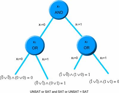
If we follow the same procedure to solve the formula but changing the order of the quantifiers we will notice that this formula is UNSAT. This is why the quantifier order is very important when solving a QBF problem.
Now we can say that a SAT problem is a QBF problem with only one existential quantifier.
Model A and Model B are two widely used QBF models for the generation of Random QBF formulas. Model A formulas are generated in a similar way to k-SAT formulas. In this model each clause has a fixed k length that is generated by randomly selecting k distinct variables from the entire set of variables and choosing if they will be positive or negative with probability one half, each clause have a j number of existential variables where j can be greater or equal to 2. The model B is similar to model A but it has a fixed set of existential variables per clause that has to be greater or equal to 2.
MINSAT and MAXSAT
MINSAT and MAXSAT are both optimization problems of SAT. They are known to be in NP-Hard which is another complexity class. Both problems are of interest to many areas of study such as computer science and electrical engineering. MAXSAT has been studied by many people. MINSAT is a less studied topic but it was of particular interest during the project as we will see.
MINSAT is defined as the optimization problem of SAT where given a set of clauses and a set of Boolean variables we have to find a truth assignment for the variables that minimizes the number of satisfied clauses. It is a very hard problem because in order to know that the given solution is the real optimum solution you have to search over the complete space of possible solutions taking a lot of time to do it.
MAXSAT is defined as given a set of clauses and a set of Boolean variables we have to find a truth assignment for the variables that maximizes the number of satisfied clauses. It is also hard because we have to search the entire space to get the optimum solution. Also this problem is more challenging for UNSAT instances than for SAT instances because in a SAT instance we know that the maximum will be the number of clauses, but for an UNSAT instance we will have to really look in the entire space. In fact, a MAXSAT problem becomes a SAT problem when we are taking about SAT instances.