|
Pulse Database Support for Efficient Query Processing Of Temporal Polynomial Models |
 |
Introduction The Pulse project develops a framework for model-based stream processing, where relational attributes are represented as mathematical models, and query processing is performed directly on the compact, symbolic forms of the model. There are numerous forms of mathematical modelling techniques, and Pulse focuses particularly on piecewise polynomials as a first step in building a practical model-based stream processing engine that investigates system design challenges in addition to the data and query model provided to end users. Polynomial-Driven Query Processing Piecewise polynomial models provide two distinctive properties for use in query processing: they facilitate random access to data at arbitrary points in time, and enable a compact representation of the data as model parameters. We consider two novel uses of models in the query execution of a stream processing engine, for predictive query processing by extrapolating data not yet seen at the system, and historical processing which interpolates data missing or simply not available (e.g. due to low sampling rates) at points of interest. Data and Query Model For predictive processing, Pulse supports declarative model specification as part of its queries via a MODEL-clause, as shown in the figure below. 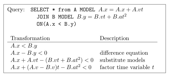
Query developers provide symbolic models defining a modeled stream attribute in terms of other attributes on the same stream and a variable t. For example in the figure above, stream A has a modeled attribute A.x defined in terms of coefficient attributes A.x and A.v. Note the self-reference to attribute A.x -- we build numerical models from actual input tuples where the values of all coefficient attributes are known, that is the right-hand side consists of bound variables. In this example, the model A.x = A.x + A.vt represents the x-coordinate a moving object as its position varies over time from some initial position. The symbolic form of a general nth degree polynomial for a modeled attribute a is: To ensure a closed operator set, we restrict the class of polynomials supported to those with non-negative exponents, since it has been shown that semi-algebraic sets are not closed in the constraint database literature [1]. In historical processing our modeling component computes coefficient attribute values internally. Pulse’s data streams contain exactly two other types of attributes, keys and unmodeled attributes. Keys are discrete, unique attributes and may be used to represent discrete enti- ties, for example different entities in a data stream of moving object locations. Unmodeled attributes are constant for the duration of a segment, as required by our time-invariant models. We omit details on the operational semantics of the core processing operators with respect to key and unmodeled processing due to space constraints. Our general strategy is to process these using standard techniques alongside the modeled attributes. Selective Operators Selective operators, such as stream filters and joins, produce outputs upon the satisfaction of a predicate comparing input attributes using one of the standard relational operators (i.e., <,≤,=,! =,≥,>). We derive our equation system by transforming predicates in a three step process. Consider the a predicate with a comparison operator R, relating two attribute x, y as xRy. Our transformation is: 1. Rewrite in difference form: x - y R 0 2. Substitute continuous model: x(t) - y(t) R 0 3. Factorize model coefficients: (x-y)(t) R 0 The above equation defines a new function, (x − y)(t), from the difference of polynomial coefficients that may be used to determine predicate satisfaction and consequently the production of results. Note that we are able to simplify the difference form into a single function by treating the terms of our polynomials independently. Depending on the comaparison operator R and the degree of the polynomial, there are various efficient methods to approach the above equation. In the case of the equality operator, standard root finding techniques, such as Newton’s method or Brent’s method [2], solve for points at which (x − y)(t) = 0. We can combine root finding with sign tests to yield a set of time ranges during which the predicate holds. 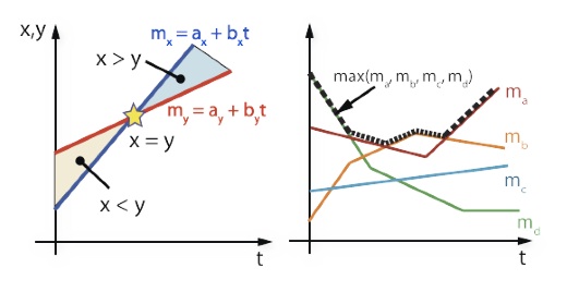 Figure 2: A geometric interpretation of the continuous transform, illustrating
predicate relationships between models for selective operators, and piecewise
composition of individual models representing the continuous internal state of a
max aggregate.
Figure 2: A geometric interpretation of the continuous transform, illustrating
predicate relationships between models for selective operators, and piecewise
composition of individual models representing the continuous internal state of a
max aggregate.
We illustrate this geometrically in the Figure 2 above. The above difference equation forms one row of our equation system. By considering more complex conjunctive predicates, we arrive at a set of difference equations of the above form that must all hold simultaneously for our selective operator to produce a result, as shown in the following equation system: 
Above, t represents a vector comprised of powers of our time variable (i.e., [t, t^2, t^3, . . . ]). The matrix D is our difference equation coefficient matrix. Under certain simplified cases, for example when R consists solely of equality predicates (as for a natural or equi-join), we may apply efficient numerical algorithms to solve the above system (such as Gaussian elimination or a singular value decomposition). A general algorithm involves solving each equation independently and determining a common solution based on intersection of time ranges. In the case of general predicates, for example including disjunctions, we apply the structure of the boolean operators to the solution time ranges to determine if the predicate holds. The equation may not have any solutions indicating that the predicate never holds within the segments’ time ranges for the given models. Consequently the operator does not produce any outputs. Aggregate Operators Min/Max Operators We focus on the scenario where a data stream consists of multiple models due to the presence of key attributes. We modify the right-hand side of the difference equation, where we now compare an input segment to the partial state maintained within the operator from aggregating over previous input segments. We denote this state as s(t), and define it as a sequence of segments: s(t) = (([tl, tu), c)1, ([tl, tu), c)_2..., ([tl, tu), c)_n), where each ([tl,tu),c)_i is a model segment defined over a time range with coefficients ci. For example with a min (or max) function, the partially aggregated model s(t) forms a lower (or upper) envelope of the model functions as illustrated in Figure 2. Thus we may write our substituted difference form as x(t) − s(t) R 0. This difference equation reflects whether the input segment updates the aggregated model within the segment’s lifespan, and we can build an equation system in the same manner as for selective operators. Sum/Avg Operators The sum aggregate has a well-defined continuous form, namely the integration operator. However, since sum and average aggregate along the temporal dimension, we handle the aggregate’s windowing behavior with window functions. These are functions parameterized over a window’s closing timestamp that return the value produced by that window. At a high level, window functions help to preserve continuity downstream from the aggregate. For a window of size w and endpoint t, we consider two possible relationships between this window and the input segments. The lifespan of a segment [tl,tu) may either match (or be larger than) the window size w, or be smaller than w. In the first case, we may compute our window results from a single segment. Specifically, a segment covering [tl, tu) may produce results for a segment spanning [tl +w, tu), since windows closed in this range are entirely covered by the segment. We define the window function for this scenario as:While the above discussion concerned a sum function, these results may easily be applied to compute window functions for averages as wfavg = wfsum/w. Error Management: Enforcing Precision Bounds Pulse supports the specification of accuracy bounds to provide users with a quantitative notion of the error present in any query result arising from differences between polynomials and the input tuples. We consider a symmetric absolute error metric and validate that Pulse's results lie within a given range of results produced by a standard stream query. A naive validation mechanism could process input tuples with both equation systems and regular stream queries and check the results. However, this performs duplicate computation, offsetting any benefits from directly processing polynomials. Our validation mechanism enforces precision bounds on polynomials at the query's inputs and completely eliminates the need for processing discrete tuples. We name this technique query inversion since it tranlates a range of output values into a range of input values by inverting the computation performed by each query operator. Some operators that are many-to-one mappings, such as joins and aggregates have no unique inverse when applied to outputs alone. Here, by inversion we mean to produce both the outputs and the inputs that caused them, not all valid inverses, and accomplish this by maintaining query lineage compactly as model segments. We use accuracy validation to drive Pulse’s curve-fitting in an online manner in predictive processing. In this scenario, Pulse only processes queries following the detection of an error. Note that accuracies may only be attributed to query results if the query actually produces a result -- given the existence of selective operators, an input tuple may yield a null result, leaving our accuracy validation in an undefined state. To account for this case, we introduce slack as a continuous measure of the query’s proximity to producing a result. We define slack as: Above, we only compute slack within valid time ranges common with the update segment causing the null (for stateful operators). Using the maximum norm ensures that we do not miss any mispredicted tuples that could actually produce results. Following a null any intermediate operator, Pulse performs slack validation, ignoring inputs until they exceed the slack range. Thus Pulse alternates between performing accuracy and slack validation based on whether previous inputs caused query results. Figure 3 provides a high-level illustration of Pulse’s internal dataflow, including the inverter component that maintains lineage from each operation and participates in both accuracy and slack bound inversion. 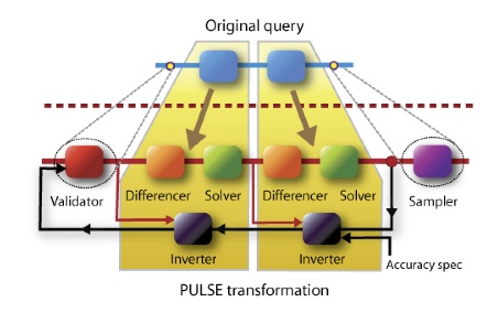 Figure 3: High level overview of Pulse’s internal dataflow. Segments are
either given as inputs to the system or determined internally, and processed as
first-class elements.
Figure 3: High level overview of Pulse’s internal dataflow. Segments are
either given as inputs to the system or determined internally, and processed as
first-class elements.
Selectivity Estimation and Adaptive Multi-Query Optimization for Continuous Function Processing Pulse’s processing strategy of solving equation systems is one of its core novelties and raises many questions how to best design an entire database system around such a query processor. In my dissertation, I implemented Pulse on top of the Borealis stream processing engine, and presented an initial solution to the broader challenge of designing architectural abstractions for model-based stream processing and error management. My dissertation also investigated statistics estimation and query optimization for equation solving. Classical databases use histograms to capture statistics on data distributions to guide a query optimizer’s decisions, however, histograms cannot trivially be applied to polynomials. Pulse’s statistics estimator uses multidimensional histograms on a parameter space of polynomial segments, and defines geometry operations on histogram bins (hypercubes) to perform selectivity estimation. Further details can be found in Chapter 3 of the dissertation below. Pulse’s optimizer uses these selectivity estimates in a novel cost model that jointly addresses operator reordering, multi-query optimization, as well as the potential for inaccurate statistics. By considering both reordering and multi-query optimization, Pulse is able to exploit a wide range of plan configurations when faced with complex selectivity scenarios. Please refer to Chapter 4 of the dissertation for more details.References [1] Gabriel M. Kuper, Leonid Libkin, and Jan Paredaens, editors. Constraint Databases. Springer, 2000. [2] Richard P. Brent. Algorithms for Minimization without Derivatives. Prentice-Hall, Englewood Cliffs, NJ, 1973. Publications:
Pulse: Database Support for Efficient Query Processing of Temporal
Polynomial Models.
Yanif Ahmad, Ph.D. thesis, Brown University, January 2009. Simultaneous Equation Systems for Query Processing on Continuous-Time Data Streams Yanif Ahmad, Olga Papaemmanouil, Ugur Cetintemel, Jennie Rogers. ICDE 2008. Declarative temporal data models for sensor-driven query processing Yanif Ahmad, Ugur Cetintemel. DMSN 2007. |