In this section we show a simple example of how to use PyGLPK to solve max flow problems.
Suppose we have a directed graph with a source and sink node, and a mapping from edges to maximal flow capacity for that edge. Our goal is to find a maximal feasible flow. This is the maximum flow problem.
This is our strategy of how to solve this with a linear program:
For the purpose of our function, we encode our capacity graph as a list of three element tuples. Each tuple consists of a from node, a to node, and a capacity of the conduit from the from to the to node. Nodes can be anything Python can hash.
The function accepts such a capacity graph, and returns the a similar list of three element tuples. The list is identical as the input list, except the capacities are replaced with the assigned flow.
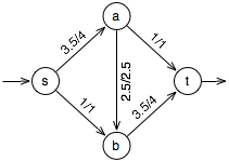
In the example graph seen at right (with given assigned/capacity weights given for the nodes), we have a source and sink 's' and 't', and other nodes 'a' and 'b'. We would represent this capacity graph as [('s','a',4), ('s','b',1), ('a','b',2.5), ('a','t',1), ('b','t',4)]
Here is the implementation of that function:
import glpk

def maxflow(capgraph, s, t):
    node2rnum = {}                      # Map non-source/sink nodes to row num.
    for nfrom, nto, cap in capgraph:
        if nfrom!=s and nfrom!=t:
            node2rnum.setdefault(nfrom, len(node2rnum))
        if nto!=s and nto!=t:
            node2rnum.setdefault(nto, len(node2rnum))

    lp = glpk.LPX()                     # Empty LP instance.
    glpk.env.term_on = False            # Stop annoying messages.
    lp.cols.add(len(capgraph))          # As many columns cap-graph edges.
    lp.rows.add(len(node2rnum))         # As many rows as non-source/sink nodes

    for row in lp.rows: row.bounds = 0  # Net flow for non-source/sink is 0.

    mat = []                            # Will hold constraint matrix entries.

    for colnum, (nfrom, nto, cap) in enumerate(capgraph):
        lp.cols[colnum].bounds = 0, cap # Flow along edge bounded by capacity.

        if nfrom == s:
            lp.obj[colnum] =  1.0       # Flow from source increases flow value
        elif nto == s:
            lp.obj[colnum] = -1.0       # Flow to source decreases flow value

        if nfrom in node2rnum:          # Flow from node decreases its net flow
            mat.append((node2rnum[nfrom], colnum, -1.0))
        if nto in node2rnum:            # Flow to node increases its net flow
            mat.append((node2rnum[nto], colnum, 1.0))

    lp.obj.maximize = True              # Want source s max flow maximized.
    lp.matrix = mat                     # Assign 0 net-flow constraint matrix.

    lp.simplex()                        # This should work unless capgraph bad.

    return [(nfrom, nto, col.value)     # Return edges with assigned flow.
            for col, (nfrom, nto, cap) in zip(lp.cols, capgraph)]
We shall now go over this function section by section!
node2rnum = {}                      # Map non-source/sink nodes to row num.
for nfrom, nto, cap in capgraph:
    if nfrom!=s and nfrom!=t:
        node2rnum.setdefault(nfrom, len(node2rnum))
    if nto!=s and nto!=t:
        node2rnum.setdefault(nto, len(node2rnum))
This is pure non-PyGLPK code, but it is doing something important for the linear program. Recall that we wanted a row for every non-source/sink node. In order to facilitate this, we first go through the capacity graph and map each node identifier (except the source and sink) to a unique integer, counting from 0 onwards.
lp = glpk.LPX() # Empty LP instance.
We create an empty LPX instance.
lp.params.msglev = 0 # Stop annoying messages.
Linear program objects contain several objects through which one can access and set some of the data associated with a linear program. One of these is the params object, which holds attributes that help control the behavior of the linear program object when running a solver, writing data, and other routines. In this case, we are setting the msglev (message level) attribute to 0, to quiet the linear program.
lp.cols.add(len(capgraph))          # As many columns cap-graph edges.
lp.rows.add(len(node2rnum))         # As many rows as non-source/sink nodes
In addition, the linear program object has two (largely identical) objects for accessing and setting traits of columns and rows, cols and rows, respectively. In this case, we are calling the add method of both objects.
Recall that we want as many structural variables (columns) as there are edges, to represent the assigned flow to edge edge. Correspondingly, we add as many columns as there are edges in the capacity graph. Also, we want as many auxiliary variables (rows) as there are non-source/sink nodes, in order to enforce the zero-net-flow constraint.
for row in lp.rows: row.bounds = 0 # Net flow for non-source/sink is 0.
In addition to being used to add rows and columns, the rows and cols objects serve as sequences, used to access row and column objects. In this case, we are iterating over all rows.
Once we have a row, we set its bounds attribute to 0 to force the row's auxiliary variable (and consequently the net flow for the corresponding node) to be zero. The bounds attribute can be assigned one or two values, depending on whether we want to assign an equality or range constraint. In this case, we want an equality constraint, and so assign the single value 0.
mat = [] # Will hold constraint matrix entries.
What's so special about an empty list? Nothing yet. However, what we are going to do is to give it elements of the linear program constraint matrix, and then set this as the linear program's constraint matrix.
The reason for this list is practical: We can set entries of the LP matrix either all at one, a whole row at a time, or a whole column at a time. None is really convenient given the structure of this problem, so we just save all the entries we want to be non-zero, and set them all at once when we have collected all of them.
Entries of the constraint matrix are given in the form of three element tuples describing the row index, column index, and the value at this location.
for colnum, (nfrom, nto, cap) in enumerate(capgraph):
    lp.cols[colnum].bounds = 0, cap # Flow along edge bounded by capacity.

    if nfrom == s:
        lp.obj[colnum] =  1.0       # Flow from source increases flow value
    elif nto == s:
        lp.obj[colnum] = -1.0       # Flow to source decreases flow value

    if nfrom in node2rnum:          # Flow from node decreases its net flow
        mat.append((node2rnum[nfrom], colnum, -1.0))
    if nto in node2rnum:            # Flow to node increases its net flow
        mat.append((node2rnum[nto], colnum, 1.0))
We are iterating over all the edges in the capacity graph. A lot is happening inside the loop, so we shall take it a piece at a time.
for colnum, (nfrom, nto, cap) in enumerate(capgraph):
Since columns correspond to edges in the capacity graph, it is convenient to just suppose that edge capgraph[i] corresponds to column lp.cols[i].
lp.cols[colnum].bounds = 0, cap # Flow along edge bounded by capacity.
Each structural variable will get the value of the flow along its corresponding edge. Naturally, we want to constrain the flow assignments to be between 0 and the edge capacity. So, we assign to the bounds attribute of the column at index colnum. Note that this is an instance of a range bound (with lower bound 0 and upper bound cap), unlike our previous equality bound.
if nfrom == s:
    lp.obj[colnum] =  1.0       # Flow from source increases flow value
elif nto == s:
    lp.obj[colnum] = -1.0       # Flow to source decreases flow value
Recall we are trying to find the maximum flow across the graph, which equals the net flow from the source. The net flow increases whenever there is flow along an edge from the source, so if the edge is from the source, we set the corresponding structural variable's objective function coefficient to 1.0 (with the effect that the assigned flow is added to the objective). Conversely, the net flow decreases whenever there is flow along an edge to the source, so if the edge is to the source, we set the corrresponding coefficient to -1.0 (with the effect that the assigned flow is subtracted from the objective).
Similar to the rows and cols attributes of linear program objects, the obj attribute also acts like a sequence. We can assign objective function coefficients through simple assignments like this. There are as many objective coefficients as there are structural variables (columns).
if nfrom in node2rnum:          # Flow from node decreases its net flow
    mat.append((node2rnum[nfrom], colnum, -1.0))
if nto in node2rnum:            # Flow to node increases its net flow
    mat.append((node2rnum[nto], colnum, 1.0))
The intent of this is very similar to our coefficients set in the objective function. We wish the net flow into a node to be zero. Correspondingly, for each edge, we add (at most) two entries to the matrix of constraint coefficients. For the "from" node of an edge, we add a -1.0 coefficient to the "from" node's corresponding row, effectively subtracting off the value of the edge's structural variable from the "from" node's auxiliary variable. For the "to" node of an edge, we add a 1.0 coefficient to the "to" node's corresponding row, effectively adding the value of the edge's structural variable to the "to" node's auxiliary variable.
The if statements are present because we only want to add this structural variables for nodes that correspond to rows, i.e., non-source/sink nodes.
This marks the end of that loop.
lp.obj.maximize = True # Want source s max flow maximized.
The obj object has an attribute maximize that controls whether we are trying to maximize or minimize the objective function. In this case, we want a maximizing assignment of flow to edges.
lp.matrix = mat # Assign 0 net-flow constraint matrix.
We set the constraint matrix to the entries that we have collected.
lp.simplex() # This should work unless capgraph bad.
Next we run the simplex algorithm to optimize this linear program. The simplex algorithm has strong theoretical ties to the max augmenting path algorith (think about the operations that are taking place in the simplex tableau), so if we have defined a valid capacity graph this should converge with no problems.
return [(nfrom, nto, col.value)     # Return edges with assigned flow.
        for col, (nfrom, nto, cap) in zip(lp.cols, capgraph)]
More or less straightforward Python code to construct the return value. For all the columns and the corresponding edges, we return the triples of "from," "to," and the variable value, which is the assigned flow. Note the use of col.value attribute to extract the primal variable value for this column.
Imagine that we run this call to find the max-flow for the given graph.
capgraph = [('s','a',4), ('s','b',1),
   ('a','b',2.5), ('a','t',1), ('b','t',4)]
print maxflow(capgraph, 's', 't')
This will produce the output
[('s', 'a', 3.5), ('s', 'b', 1.0), ('a', 'b', 2.5),
 ('a', 't', 1.0), ('b', 't', 3.5)]
corresponding to the flow shown in the graph.