Moser's Algorithm and the Lovász Local Lemma

In this survey, we’ll examine the Lovász Local Lemma (LLL), a cornerstone of the probabilistic method, through the lens of theoretical computer science. This powerful tool was developed in the 70s by Hungarian mathematicians Lovász and Erdős to guarantee the existence of certain combinatorial structures¹, and it has since been borrowed by computer scientists to prove results about satisfiability problems, graph colorings, tree codes, integer programming, and much more².

For quite some time, this method remained entirely non-constructive, until a quest to constructify the LLL began in the 90s³. For a while, all results required rather significant assumptions, but breakthrough work by Moser and Tardos in 2009 proved the efficacy of a suprisingly simple randomized search algorithm⁴ ⁵. This post will describe an elegant proof of Moser’s algorithm using the method of entropy compression. If you are already familiar with the LLL, you may want to skip to the third section.

The Probabilistic Method

The probabilistic method is a useful non-constructive technique that was pioneered by Paul Erdős in the 40s to prove foundational results in Ramsey theory⁶. In general, this setup begins with a search space $\Omega$ (usually large and finite) and a set $\mathcal{B}$ of flaws that we aim to avoid. Specifically, each $B \in \mathcal{B}$ is a subset of $\Omega$ whose objects share some undesired trait, and we are searching for a flawless object $\sigma \in \Omega \setminus \cup_{B \in \mathcal{B}} B$. The probabilistic approach to this search is to place a probability measure on $\Omega$, so that $\mathcal{B}$ corresponds to a set of “bad” events. Then, we can borrow tools from probability theory to prove that the probability of no bad events occuring, \[ \Pr[\land_{B \in \mathcal{B}} \overline{B}] = 1 - \Pr[\lor_{B \in \mathcal{B}} B], \] is strictly positive, certifying the existence of a flawless object. While this approach is often just a counting argument in disguise, it has proven to be quite fruitful and has helped combinatorialists avoid redeveloping existing probabilistic machinery. The classic applications of this method are to graph coloring, but $k$-SAT seems better suited to a computer science audience.

Let $\varphi$ be a Boolean formula in conjunctive normal form (CNF) with $n$ variables, $m$ clauses, and $k$ variables in each clause. The $k$-SAT decision problem asks, given such a $\varphi$, whether there exists an assignment of variables satisfying all of its clauses. We will diverge slightly from the traditional $k$-SAT definition by requiring that the variables of each clause are distinct. In this case, our search space \[ \Omega = \{\text{True}, \text{False}\}^n \] consists of variable assignments, and our flaws \[ B_i = \{ \sigma \in \Omega \mid \text{$\sigma$ violates clause $i$ of $\varphi$} \}, \quad i = 1, \dots, m \] correspond to violated clauses. We will simply select the uniform probability measure over $\Omega$, i.e. flip a fair coin to determine the assignment of each variable. With this choice, \[ \Pr[B_i] = \frac{1}{2^k}, \] since there is a single assignment of the $k$ variables in a CNF clause which cause it to be violated.

Perhaps the most generic tool we have at our disposal is the union bound. In the case of $k$-SAT, this guarantees that a satisfying assignment exists when the number of clauses is small. Specifically, if $m < 2^k$, we have \[ \Pr[\land_{i=1}^m \overline{B_i}] = 1 - \Pr[\lor_{i=1}^m B_i] \geq 1 - \sum_{i=1}^m \Pr[B_i] = 1 - m 2^{-k} > 0, \] as desired. Another simple case is when all of the clauses are disjoint; then, the $B_i$ events are independent and \[ \Pr[\land_{i=1}^m \overline{B_i}] = \prod_{i=1}^m \Pr[\overline{B_i}] = (1 - 2^{-k})^m > 0. \] In general, we have the following when each bad event occurs with at most probability $p$.

Method	Assumptions on …	Sufficient condition for flawless object
Union bound	n/a	$p < 1/n$
Independence	Global event structure	$p < 1$
???	Local event structure	$p < \,?$

As the final row suggests, it is natural to ask whether one can interpolate between these two results with assumptions on local event structure.

The Lovász Local Lemma

This question was given an affirmative answer in the 70s when Lászlo Lovász developed his local lemma to establish a hypergraph colorability result⁷. We will first describe the so-called symmetric LLL, which is often applied when the bad events are identical up to some (measure-preserving) permutation of the objects.

Theorem (Symmetric LLL)

Let $\mathcal{B}$ be a set of events such that each occurs with probability at most $p$ and is mutually independent from all but at most $d$ other events. Then, if $ep(d + 1) \leq 1$, $\Pr[\land_{B \in \mathcal{B}} \overline{B}] > 0$.

For $d \geq 1$, this condition was later relaxed by Shearer to $epd \leq 1$⁸. The dependency bound $d$ serves as a characterization of local event structure, and this result fits into table as $p < 1/(ed)$, nearly interpolating smoothly between independence and the union bound. Let’s examine the consequences of the LLL for $k$-SAT.

Example

Suppose that each variable of our $k$-CNF formula appears in at most $2^k/(ke)$ clauses. Then each clause can share variables with at most $k \cdot 2^k/(ke) = 2^k/e$ clauses, giving a dependency bound of $d = 2^k/e$ between our bad events. Since $p = 2^{-k}$, $epd = 1$, and the LLL condition (barely) holds, guaranteeing the existence of a satisfying variable assignment.

In the asymmetric case, we will require a more nuanced description of event structure.

Definition (Dependency Graph)

Let $\mathcal{E}$ be a set of events in a probability space. A graph with vertex set $\mathcal{E}$ is called a dependency graph for $\mathcal{E}$ if each event is mutually independent from all but its neighbors.

Example

Consider the 2-CNF formula $\varphi = (x_1 \lor x_2) \land (\neg x_2 \lor x_3) \land (x_3 \lor \neg x_4)$. Then, we have three bad events to avoid; $B_1$ associated with $x_1 \lor x_2$, $B_2$ associated with $\neg x_2 \lor x_3$, and $B_3$ corresponding to $(x_3 \lor \neg x_4)$. The following are valid dependency graphs for this event set. Example dependency graphs.

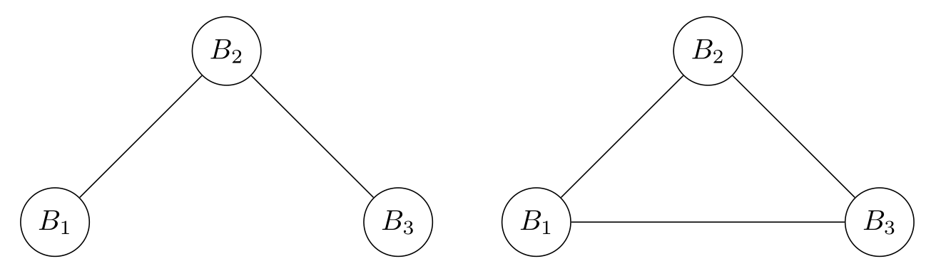
Remark

In the case of $k$-SAT, there is a unique edge-minimum dependency graph with edges connecting events whose corresponding clauses share variables; however, there is no canonical dependency graph for general event sets. Furthermore, when we move from an event set to a dependency graph, we lose information about the events.

Now, we can state the LLL in its general form, where we let $N_G(v)$ denote the neighbors of vertex $v$ in graph $G$.

Theorem (Asymmetric LLL)

Given a set of bad events $\mathcal{B}$ with dependency graph $G$, if there exists some $x \in (0,1)^{\mathcal{B}}$ such that \[ \Pr[B] \leq x_B \prod_{C \in N_G(B)} (1 - x_C) \quad \forall B \in \mathcal{B}, \] then $\Pr[\land_{B \in \mathcal{B}} \overline{B}] > 0$.

Remark

We can recover the symmetric case as a corollary by setting each $x_B = 1/(d+1)$. Indeed, this choice of $x$ results in the requirement \[ \Pr[B] \leq \frac{1}{d+1}\left(1 - \frac{1}{d+1}\right)^d, \] which is implied by the condition $ep(d+1) \leq 1$, since \[ \frac{1}{e} \leq \left( 1 - \frac{1}{d+1} \right)^d. \]

We omit a proof of the asymmetric LLL, though it essentially follows from inductive applications of Bayes’ Theorem.

Variable LLL and Moser’s Algorithm

In most applications of the LLL (for instance, $k$-SAT and graph coloring), the bad events of interest are generated by a finite set of independent random variables. To capture this richer structure, we introduce the following.

Definition (Event-Variable Bigraph)

Let $\mathcal{B}$ be a set of events and $\mathcal{X}$ be a set of mutually independent random variables such that each event $B \in \mathcal{B}$ is completely determined by a subset of variables $\operatorname{vbl}(B) \subset \mathcal{X}$. We define the event-variable bigraph of this system to be the bipartite graph $H = (\mathcal{B} \cup \mathcal{X}, E)$ with $B,X \in E$ if and only if $X \in \operatorname{vbl}(B)$.

Definition (Base Dependency Graph)

Given such an event-variable bigraph $H = (\mathcal{B} \cup \mathcal{X}, E)$, we define its base dependency graph $G_H = (\mathcal{B}, E')$, where $B,B' \in E'$ if and only if $\operatorname{vbl}(B) \cap \operatorname{vbl}(B') \neq \emptyset$.

Observe that $G_H$ is a dependency graph for $\mathcal{B}$ (in fact, its edge-minimum dependency graph as long as no variable set is unecessarily large).

Example

Recall the previous the 2-CNF formula $\varphi = (x_1 \lor x_2) \land (\neg x_2 \lor x_3) \land (x_3 \lor \neg x_4)$ with corresponding bad events $B_1, B_2, B_3$. This system admits the following event-variable bigraph, Example dependency graphs.
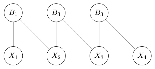
where $X_i$ is the random variable corresponding to the assignment of $x_i$.

With this variable formulation well-defined, we are now prepared to constructify the LLL. The algorithm which I will present was published by Robin Moser in 2008⁹ and extended to the general variable setting in 2009 alongside his advisor Gábor Tardos¹⁰. Their approach was a major breakthrough over previous work, which required significant assumptions on top of this variable structure. Particularly suprising was its simplicity; the algorithm is perhaps the simplest non-trivial procedure one could imagine to find a satisfying variable assignment. Specifically, given a set $\mathcal{B}$ of bad events generated by a finite set of random variables $\mathcal{X}$, Moser’s algorithm finds an assignment of the random variables such that all of the bad events are avoided, as follows.

Algorithm (Resample)

Input: Finite event-variable bigraph $(\mathcal{B} \cup \mathcal{X}, E)$, procedure for sampling from each random variable $X \in \mathcal{X}$
Output: Assignments $v = (v_X)_{X \in \mathcal{X}}$ of variables such that no event $B \in \mathcal{B}$ occurs

Randomly sample assignment $v_X \sim X$ for each variable $X \in \mathcal{X}$
While $\exists$ event $B \in \mathcal{B}$ which occurs under assignments $v$
Resample $v_X \sim X$ for each variable $X \in \operatorname{vbl}(B)$
Return $v$

Of course, assumptions on the events and their structure is necessary for Resample to run efficiently (or even to just terminate). Initially, Moser and Tardos proved good performance under asymmetric LLL conditions¹¹.

Theorem (Running time of Resample)

If there exists some $x \in (0,1)^{\mathcal{B}}$ such that \[ \Pr[B] \leq x_B \prod_{C : \operatorname{vbl}(B) \cap \operatorname{vbl}(C) \neq \emptyset} (1 - x_C) \quad \forall B \in \mathcal{B}, \] then Resample finds an assignment of variables such that no event occurs in at most \[ \sum_{B \in \mathcal{B}} \frac{x_B}{1 - x_B} \] expected resampling steps.

Entropy Compression

In a 2009 blog post, Terence Tao presented a particularly elegant analysis of this algorithm, inspired by a talk Moser gave at STOC. His write-up coined the term entropy compression, a clever principle for bounding the running time of an algorithm using a reduction from data compression. To describe this method, we first introduce some fundamental definitions and results from information theory. See David MacKay’s textbook for a more comprehensive reference.

Definition (Information Content)

The information content, or surprisal, of an event $E$ is given by \[ I(E) = -\log \Pr(E), \] with the logarithm taken in base 2.

This notion captures the fact that we learn more from the occurence of a rare event than a frequent event.

Definition (Entropy)

The (Shannon) entropy of a discrete random variable $X$ with finite support $\mathcal{X}$ is defined as \[ H(X) = \mathbb{E}_{x \sim X} I(X = x) = - \sum_{x \in \mathcal{X}} \Pr[X = x] \log(\Pr[X = x]). \]

Entropy captures the expected amount of information obtained from measuring a random variable. Our exact choices of functions for $I$ and $H$ are supported by an elegant connection to coding theory.

Definition (Uniquely Decodable Codes)

For two alphabets (i.e. sets of symbols) $\Sigma_1$ and $\Sigma_2$, a code is function $C: \Sigma_1 \to \Sigma_2^*$ mapping each symbol of $\Sigma_1$ to a string of symbols over $\Sigma_2$. The extension of $C$ is the natural homomorphism it induces from $\Sigma_1^*$ to $\Sigma_2^*$, mapping each $s_1s_2 \dots s_n \in \Sigma_1^*$ to $C(s_1)C(s_2) \dots C(s_n) \in \Sigma_2^*$. A code is uniquely decodable if its extension is injective.

The following result establishes the limits of noiseless data compression in terms of entropy.

Theorem (Shannon’s Source Coding Theorem, Simplified)

For a discrete random variable $X$ with finite support $\mathcal{X}$, let $f:\mathcal{X} \to \{0,1\}^*$ be a uniquely decodable code. Then, we can bound the expected length of the codeword $f(X)$ from below by the entropy of $X$, i.e. \[ \mathbb{E}|f(X)| \geq H(X). \]

Of particular interest to computer scientists is the following example.

Example

In particular, if $X \sim U(\{0,1\}^r)$ is an $r$-bit string selected uniformly at random, then \[\begin{align*} \mathbb{E}|f(X)| \geq H(X) &= - \sum_{x \in \{0,1\}^r} \Pr[X = x] \log(\Pr[X = x])\\ &= -\log(1/2^r) = r \end{align*}\] for any uniquely decodable $f:\{0,1\}^r \to \{0,1\}^*$. Essentially, this means that $r$ random bits cannot be noiselessly compressed into fewer than $r$ bits in expectation.

Finally, we are prepared to outline Tao’s entropy compression principle.

Theorem (Entropy Compression)

Consider an algorithm $\mathcal{A}$ with access to a stream of bits sampled independently and uniformly at random. Suppose that $\mathcal{A}$ proceeds though a sequence of steps $t = 0,1,\dots$ until (potentially) terminating, such that the following hold for any input:

$\mathcal{A}$ can be modified to maintain a bit string $L_t$ logging its history after each step $t$, such that the random bits read so far can be recovered from $L_t$;
- The computational cost (or even computability) of this history log modification is irrelevant.
- The precise notion of recovery is a bit nuanced¹² – we will elaborate within the proof.
$L_t$ has length at most $\ell_0 + t\Delta \ell$ after step $t$;
$r_0 + t\Delta r$ random bits have been read after step $t$.

If $\Delta \ell < \Delta r$, then the step after which $\mathcal{A}$ terminates is at most \[ \frac{\ell_0 - r_0}{\Delta r - \Delta \ell} \] in expectation.

Proof

Fix any input to the algorithm. For each ($r_0 + t\Delta r$)-bit string $y$, sufficient to run the algorithm up to step $t$, let $s = s(y) \leq t$ denote the step at which the algorithm terminates when its random stream is replaced by the fixed string $y$. Then, we denote the final history log by $L_s(y)$ and let $z(y)$ be the suffix of $y$ consisting of the $(t - s)\Delta r$ bits unused due to early termination. Making the notion of recovery for the history logging protocol precise, we require that the code $f:\{0,1\}^{r_0 + t\Delta r} \to \{0,1\}^*$ defined by the concatenation \[ f(y) = L_s(y) \circ z(y) \] is uniquely decodable, for all $t$. This is a slightly technical condition, but it will not be an obstacle for our analysis of Moser’s algorithm. Now, supplying random bits $Y \sim U(\{0,1\}^{r_0 + t\Delta r})$ to the algorithm, resulting in a run to step $S = s(Y)$, we find that \[ |f(Y)| = |L_S(Y)| + (t - S)\Delta r \leq \ell_0 + S \Delta \ell + (t - S)\Delta r. \] Next, we use the source coding bound of $\mathbb{E}|f(Y)| \geq H(Y)$ and rearrange to obtain \[ \mathbb{E}[S] \leq \frac{\ell_0 - r_0}{\Delta r - \Delta \ell}. \] Since $\mathcal{A}$ always completes its zeroth step, source coding also requires that $\ell_0 \geq r_0$, ensuring that the previous bound is always sensical (non-negative). Finally, if $T$ denotes the terminating step of the algorithm when provided with a stream of random bits (with the convention that $T=\infty$ when the algorithm fails to halt), we see that $S = \min\{t,T\}$. Since our bound on $\mathbb{E}[S]$ is independent of $t$, it also applies to $\mathbb{E}[T] = \lim_{t \to \infty}\mathbb{E}[S]$, as desired.

Essentially, if our algorithm is logging fewer bits than it reads at each step, it cannot progress too far in expectation without acting as an impossibly good compression protocol. Note that the identity protocol, which simply logs the random bits read so far without modification, satisfies our unique decodability requirement and can be appended to any algorithm. In this case, $\Delta \ell = \Delta r$, and the entropy compression bound means that an algorithm admitting a better protocol cannot continue indefinitely.

Remark

Alternatively, one can formalize this analysis using Kolmogorov complexity to get a bound with high probability, as described in this blog post by Lance Fortnow.

Analysis of Moser’s Algorithm

Now, we will apply our new found principle to analyze Moser’s algorithm. For conciseness, we will restrict ourselves to the $k$-SAT example and consider a slightly modified procedure. Recall that we are requiring $k$-CNF formulas to have exactly $k$ distinct variables in each clause.

Algorithm (Resample2)

Input: $k$-CNF formula $\varphi$
Output: Assignments $x \leftarrow$ solve($\varphi$) such that $\varphi(x)$ holds

solve($\varphi$)
Randomly assign each $x_i$ true or false with equal probability
While $\exists$ unsatisfied clause $C$
x $\leftarrow$ fix($x, C, \varphi$)
Return $x$
fix($x, C, \varphi$)
Randomly resample each $x_i \in C$
While $\exists$ unsatisfied clause $D$ sharing a variable with $C$
x $\leftarrow$ fix($x, \varphi, D$)
Return $x$

This algorithm is very similar in spirit to Resample, with the added recursive step of fixing nearby clauses before continuing to other unsatisfied clauses. We will prove efficient running time bounds for this algorithm assuming slightly relaxed symmetric LLL conditions, under a model of computation where sampling a single random bit takes $O(1)$ time.

Theorem (Running Time of Resample2)

Let $\varphi$ be a $k$-CNF formula with $n$ variables and $m$ clauses. If each clause of $\varphi$ shares variables with at most $2^{k - C}$ other clauses, then Resample2 runs in $O(n + mk)$ expected time, where $C$ is an absolute constant.

Remark

Note that $C = \log_2(e)$ would match the symmetric LLL conditions exactly.

Proof

To apply entropy compression, we must first divide each run of Resample2 into steps. We let the initial assignments of solve comprise step 0 and let each clause resampling by fix consistitute an additional step. Our key observation is that only one assignment of the relevant $k$ variables can cause a $k$-CNF clause to be violated and require fixing. Thus, given a stack trace of an algorithm run, we can work backwards from the final string $x$ to recover the sampled random bits. For example, suppose that $x_1 \lor \neg x_2 \lor x_3$ was the last clause of a 3-CNF formula to be fixed by Resample2. Then, the final assignments of these variables give the last three bits sampled, and their previous assignments must have been (False, True, False).

Now, we use the dependency bound of $d \leq 2^{k-C}$ to construct an efficient history logging protocol. Every history log will begin with $n$ bits specifying the current variable assignment. Then, we mark the clauses which were fixed by non-recursive calls from solve. Since there are $m$ clauses in total, such a subset can be described by $m$ bits, with each bit specifying the membership status of a particular clause. Next, for each clause, we fix an ordering of the $\leq d + 1$ clauses it shares variables with (including itself). Then, for the clauses of recursive calls to fix, we can simply log their index with respect to the “parent” clause which called them, requiring at most $\lceil \log(d + 1) \rceil + O(1)$ bits (with constant $O(1)$ information used to keep track of the recursion stack). Reading through such a log as part of a larger string, one can determine when the log has terminated and how many steps were completed by the run it encodes, so it is simple enough to show that our unique decodability condition holds.

Thus, if the algorithm has called fix $t$ times, our log has length at most $n + m + t(\log(d) + O(1))$. However, we have sampled $n$ bits for the initial assignments and $k$ for each call to fix, giving a total of random $n + kt$ bits. By the dependency bound, the history log “write rate” of $\log(d) + O(1) = k - C + O(1)$ bits per step is less than the random bit “read rate” of $k$ bits per step, for sufficiently large $C$. Thus, our entropy compression principle states that the number of calls to fix is at most $O(n + m - n) = O(m)$ in expectation. The total number of random bits sampled by Resample2 is therefore $O(n + mk)$ in expectation, as desired.

Many lower bounds in theoretical computer science are proven using information theory, but Moser was the first, to my knowledge, to provide an upper bound using such methods. The key ingredient of his original proof was that of a witness tree, similar in spirit to our history log above. Although this technique was quite novel at the time, Tao observed that it could framed in a more familiar light. Algorithm analysis often exploits monotonic properties that consistently increase over the course of an algorithm. If one can ensure that there is a constant increase at each step and that the property is bounded from above, then this gives an upper bound on the number of steps taken by the algorithm (common examples of monotonic properties include cardinalities, weights, densities, and energies). In this case, we essentially¹³ have that the ratio of entropy to output plus history log length is bounded by one and increases by a constant amount with each (expected) step, ensuring termination. With this interpretation, “entropy compression” is a very natural description of our analysis method.

Remark

As a final aside, I’d like to promote the excellent Budapest Semesters in Mathematics program, where I first learned about the LLL in András Gyárfás’s class on the combinatorics of finite set systems.

Paul Erdős and László Lovász. “Problems and Results on 3-Chromatic Hypergraphs and Some Related Questions”.↩
Michael Molloy. “The Probabilistic Method”.↩
Jószef Beck. “An Algorithmic Approach to the Lovász Local Lemma”.↩
Robin A. Moser. “A Constructive Proof of the Lovász Local Lemma”.↩
Robin A. Moser and Gábor Tardos. “A Constructive Proof of the General Lovász Local Lemma”.↩
Noga Alon and Joel H. Spencer. “The Probabilistic Method”.↩
Paul Erdős and László Lovász. “Problems and Results on 3-Chromatic Hypergraphs and Some Related Questions”.↩
James B. Shearer. “On a Problem of Spencer”.↩
Robin A. Moser. “A Constructive Proof of the Lovász Local Lemma”.↩
Robin A. Moser and Gábor Tardos. “A Constructive Proof of the General Lovász Local Lemma”.↩
Robin A. Moser and Gábor Tardos. “A Constructive Proof of the General Lovász Local Lemma”.↩
In fact, I was confused enough to ask about it on Math Overflow, where Tao answered my (misguided) question himself!↩
Formalizing this in the proof required some care, capping the length of the random stream, but the description is morally correct.↩

Method	Assumptions on …	Sufficient condition for flawless object
Union bound	n/a	\(p < 1/n\)
Independence	Global event structure	\(p < 1\)
???	Local event structure	\(p < \,?\)