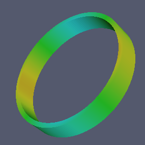

In this tutorial, we will compute devi>e characteristics for a ring resonator. We will write a short Lua script to describe the geometry and material properties. Then we will use built-in solvers to find the lowest vibrational frequency of the resonator corresponding to a particular azimuthal number. We will also compute Bryan's factor, quality factor due to thermoelastic damping, and their sensitivities to the design parameters.
Working with axisymmetric objects enables us to use two dimensional cross section in \((r,z)\)-plane and the cylindrical coordinates for our computations.
We can think of the geometry of the cross section composed of multiple blocks tied together. In order to create the mesh, we will use mapped_block generator. Mapped block generator maps \((x,y) \in [-1,1]\times[-1,1]\) to the real block in the mesh. We have to write this mapping function based on the geometry we want to describe.
We will add a require statement at the top of our script to use library functions. This is similar to #include in C language.
require "mapped_block"The program recognizes materials using unsigned integer ids. We prefer to give a name to each material which will make it easier to refer it later. For this purpose we will create a global variable and initialize it to a unique unsigned integer. Let the ring be made of material \(0\) which we will call SILICON.
We can add materials to our context by providing the following keys in a table: id unsigned integer unique to each material, E is Young's modulus, nu is Poisson's ratio, rho is material density, kappa is thermal conductivity, alpha is thermal coefficient of expansion, cv is specific heat at constant volume, and T0 is the material temperature. We use MKS units.
T0 = 300

SILICON = {
   id    = 0, -- unique material id
   E     = 165e9,
   nu    = 0.26,
   rho   = 2330.0,
   kappa = 142,
   alpha = 2.6e-6,
   cv    = 710,
   T0    = T0 } -- T0 on the lhs is a key in material table,
                -- T0 on the rhs is the value from global variable T0
We will describe our ring resonator as a thin cylindrical shell. The cross section of this object is a thin rectangle elongated in the axial direction. The boundaries are straight lines. We can achieve a representation of this rectangular region by appropriately scaling the domain \([-1,1]\times[-1,1]\).
function ring_mesh_generator(R,h,L)
   local function map(x,y)
      local r = R + x*h/2; -- notice the shift corresponding to the radius
      local z = y*L/2
      return r,z
   end

   -- mapped block will return a single block with 8x40 cells
   return  mapped_block {
      phi = map,          -- mapping function
      material = SILICON, -- material type
      m = 8,              -- divisions in r
      n = 40}             -- divisions in z
end
Now we can define a Problem object which will form a context for our computations. We start by specifying the geometric design parameters, and also provide the temperature in Kelvins which will be used in computation of quality factor. The construction of the Problem context is done by passing a table of key-value pairs. Within this context, params refers to the geometric design parameters, and meshgen refers to the mesh generator function. Notice that the list of parameters are in the order our mesh generator expects. m specifies the azimuthal number.
   R  = 2e-3
   h  = 1.6e-4
   L  = 7e-4

   P = Problem:create{ params = {R,h,L},   -- mesh generator design parameters
                    m      = 2,         -- azimuthal number
                    meshgen= ring_mesh_generator }


P:add_material(SILICON)Slightly modified meshes are generated using stepsizes provided, and they are used to compute the mesh gradient using two sided finite difference approximation. We need this call to perform sensitivity analysis.
P:mesh_gradient();We can output the mesh as follows:
P:write_svg("ring.svg") -- in Scalable Vector Graphics format
P:write_eps("ring.eps") -- in Encapsulated PostScript formatAll boundaries are free for the displacement variables, and isolated for the temperature variable. We will introduce how to describe the boundary conditions in the second tutorial. For now accept that the following code snippet will do the job.
function free(r,z,d) return false end
P:set_boundary_conditions{  radial = {free},
                           angular = {free},
                             axial = {free},
                       temperature = {free}  }
In order to solve for the device characteristics and sensitivities, we just call a couple of functions. Assembly and computations of values are performed based on their dependency.
f0 = P:get_eigenfrequency()     -- Eigenfrequency in Hz
BF = P:get_bryans_factor()      -- Bryan's factor
Q  = P:get_quality_factor()     -- Q_TED

print("Frequency      : "..f0)
print("Bryan's factor : "..BF)
print("Quality factor : "..Q )
To compute the sensitivities to design parameters, we pass the index of the corresponding parameter in the prototype of the mesh generator. In our example, function ring_mesh_generator(R,h,L) \(R\) corresponds to index 0, \(h\) to index 1 and \(L\) to index 2. So, if we want to compute \(\partial f_0/\partial R\), \(\partial BF/\partial h\) and \(\partial Q/\partial L\), we use the following functions.
df0dR = P:eigenfrequency_sensitivity(0)
dBFdh = P:bryansfactor_sensitivity(1)
dQdL  = P:qualityfactor_sensitivity(2)

print("df0dR : "..df0dR)
print("dBFdh : "..dBFdh)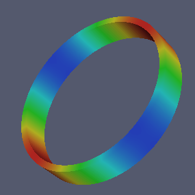
print("dQdL : "..dQdL )We can create pictures of radial \(u_r\), angular \(u_{\theta}\) and axial \(u_z\) displacement fields on the two dimensional cross section using the function write_svg. We have to specify a filename and which field we want to plot.
P:write_svg{"disp0.svg"; field=0}
P:write_svg{"disp1.svg"; field=1}
P:write_svg{"disp2.svg"; field=2}
We can also create three dimensional pictures using write_inp function. Its usage is similar to write_svg. However the output format is UCD (.inp) which can be visualized using Paraview.
P:write_inp{"disp0.inp"; field=0}
P:write_inp{"disp1.inp"; field=1}
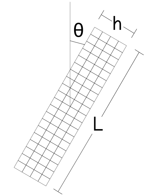
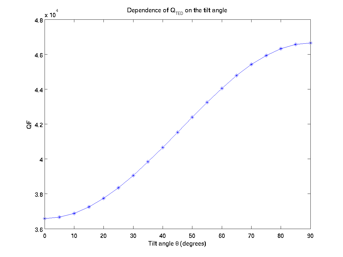
P:write_inp{"disp2.inp"; field=2}In the tutorial, we considered the ring to be a thin cylinder. Could you add a tilt \(\theta\) to the cross section so that the ring becomes a cut from a cone? Could you write a for loop to investigate how \(f_0\), \(BF\), and \(Q\) change as a function of \(\theta\)?
require "mapped_block"
T0 = 300
SILICON = {
id = 0, -- unique material id
E = 165e9,
nu = 0.26,
rho = 2330.0,
kappa = 142,
alpha = 2.6e-6,
cv = 710,
T0 = T0 } -- T0 on the lhs is a key in material table,
-- T0 on the rhs is the value from global variable T0
function tilted_ring_mesh_generator(R,h,L,theta)
local function map(x,y)
local xx = x*h/2
local yy = y*L/2
local r = R + xx*cos(theta) + yy*sin(theta)
local z = L/2 - xx*sin(theta) + yy*cos(theta)
return r,z
end
return mapped_block{
phi = map,
material = SILICON,
m = 2,
n = 10 }
end
R = 2e-3
h = 1.6e-4
L = 7e-4
-- Opens a file in write mode for the results
f = io.open("tilted_results.txt","w")
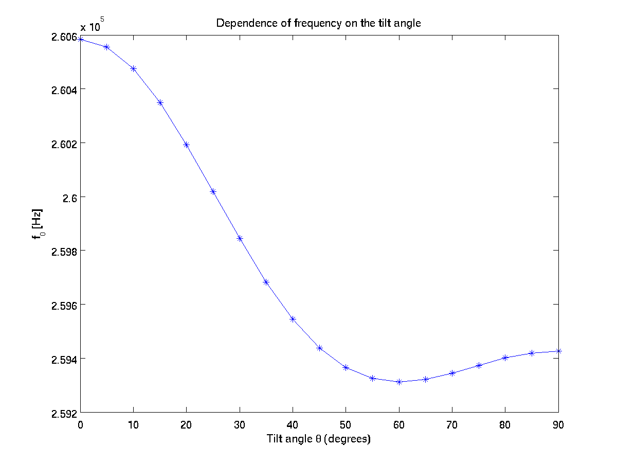
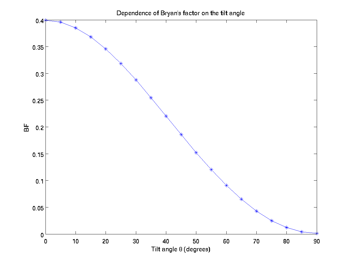
-- Sweeps the tilt angle in 5 degree steps from 0 to 90.
for deg=0,90,5 do
theta = deg*pi/180
P = Problem:create{ params = {R,h,L,theta},
meshgen = tilted_ring_mesh_generator,
refinement = 3, -- refines the mesh returned by the
-- mesh generator 3 times
m = 2 }
P:add_material(SILICON)
P:mesh_gradient() -- computes finite difference mesh gradient
P:write_eps("tilted_ring.eps")
function free(r,z,d) return false end
P:set_boundary_conditions{ radial={free},angular={free},
axial={free},temperature={free}}
f0 = P:get_eigenfrequency()
BF = P:get_bryans_factor()
Q = P:get_quality_factor()
-- Writes the value f0, BF, and Q to file
f:write(deg.." "..f0.." "..BF.." "..Q.."\n")
end
f:close()The saved results are plotted in files ex1_f0.png, ex1_bf.png and ex1_qf.png.
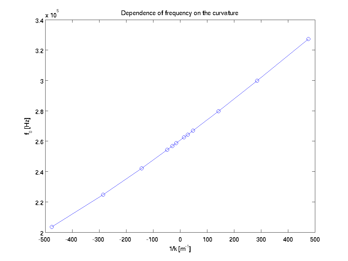
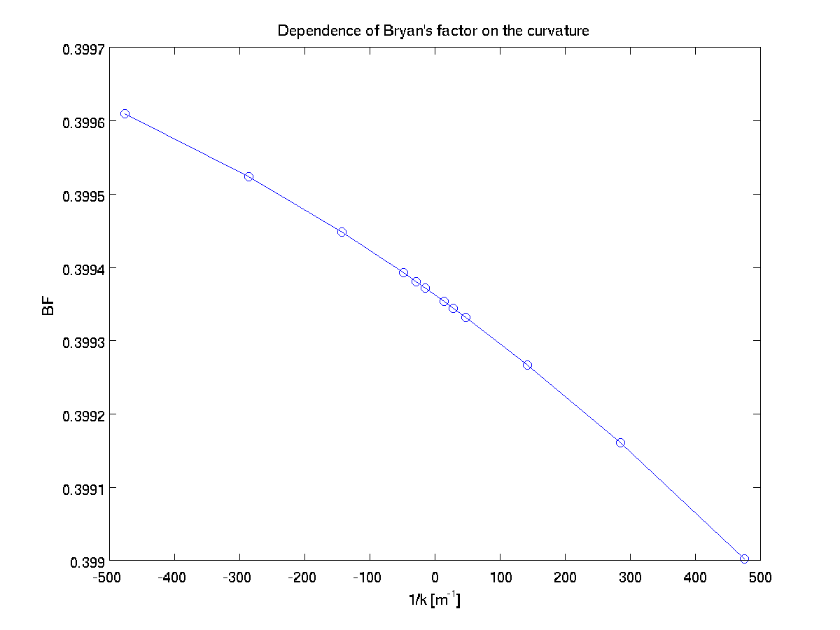
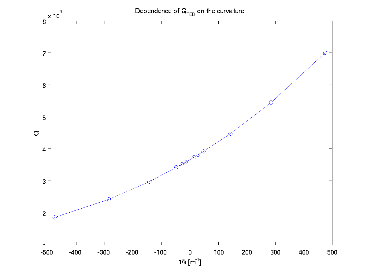
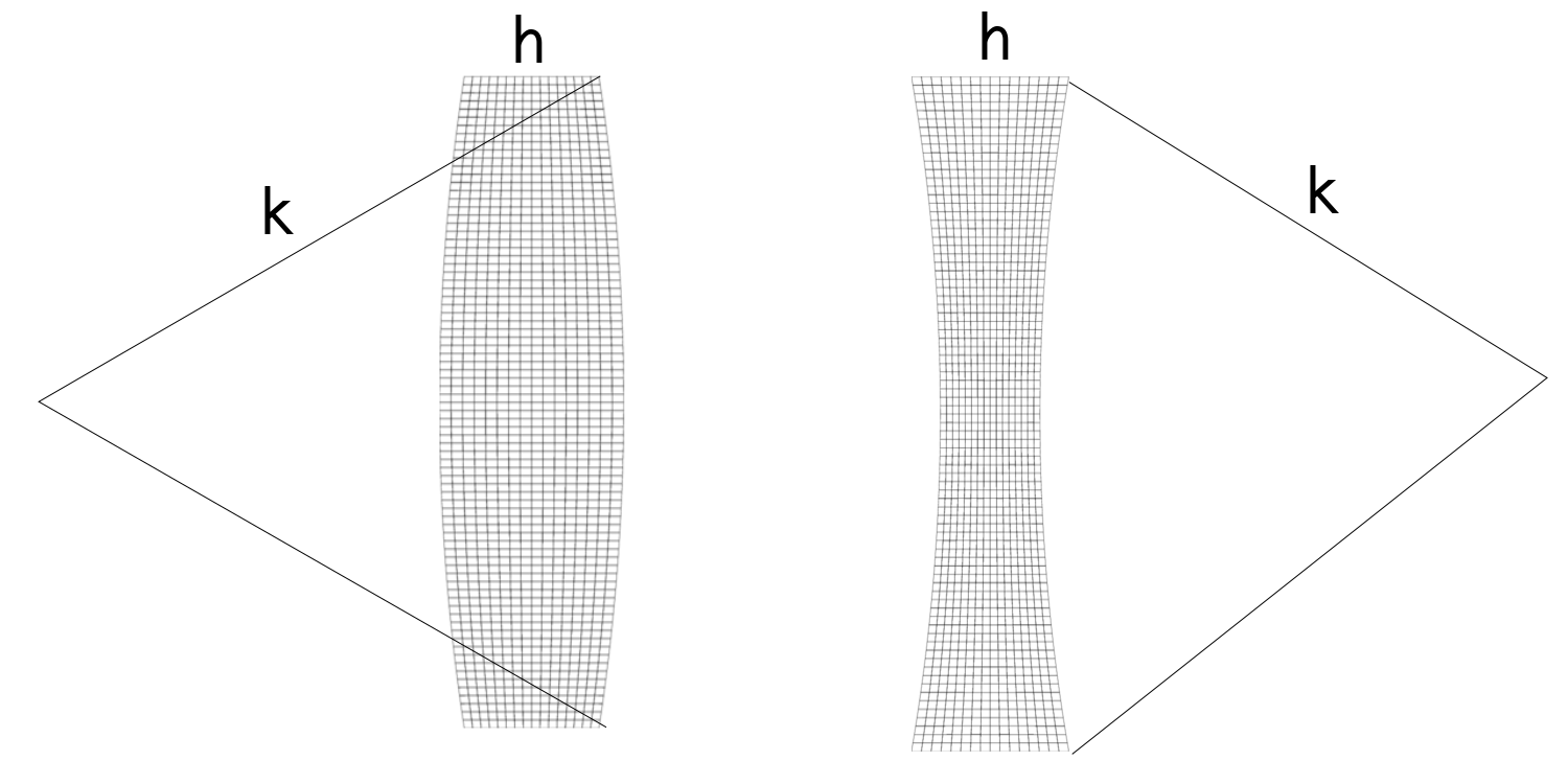
In the tutorial we considered a rectangular cross section. What happens if the sides were a bit bulged? Could you modify the mesh generator to include the radius of curvature \(k\) on both inner and outer sides? Could you compare the concave and convex situations? How much does Bryan's factor change with a slight curvature effect for a rectangular cross section?
require "mapped_block"

T0 = 300

SILICON = {
   id    = 0, -- unique material id
   E     = 165e9,
   nu    = 0.26,
   rho   = 2330.0,
   kappa = 142,
   alpha = 2.6e-6,
   cv    = 710,
   T0    = T0 } -- T0 on the lhs is a key in material table,
                -- T0 on the rhs is the value from global variable T0
We have to change the mesh generator. There are various ways to write a mapping function. Here we will assume that z-coordinate of mesh points are not effected by bulging. In radial direction we will consider the effective thickness to be larger than h. Using the figure below, we can compute the relevant lengths.
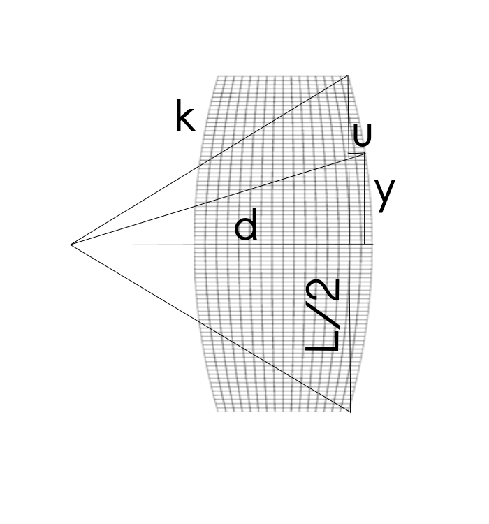
function bulged_ring_mesh_generator(R,h,L,k)
   local function map(x,y)
      local d  = sqrt(k*k-L*L/4)
      local yy = y*L/2
      local u  = sqrt(k*k-yy*yy)-d
      if k < 0 then u = -u end
      local hy = h + 2*u
      local xx = x*hy/2
      local r  = R   + xx
      local z  = yy

      return r,z
   end

   return mapped_block{
            phi = map,
            material = SILICON,
            m = 2,
            n = 10    }
end
R = 2e-3
h = 1.6e-4
L = 7e-4
-- Open a file in write mode for the results
f = io.open("bulged_results.txt","w")
For various ratios \(n=k/L\), we will compute results. nvals table provides some samples for both concave and convex situations in order of increasing curvature.
nvals = {-3,-5,-10,-30,-50,-100,100,50,30,10,5,3}
for i,n in ipairs(nvals) do

k = L*n
The rest of the code is similar to the tutorial. After computing the results, we will write them to a text file in order to process further with your favorite graphing tool.
P = Problem:create{ params  = {R,h,L,k},
                 meshgen = bulged_ring_mesh_generator,
                 refinement = 3,
                 m       = 2 }

P:add_material(SILICON)

P:mesh_gradient() -- computes finite difference mesh gradient

-- this will output the mesh with a filename indexed with i
P:write_eps("bulged_ring_"..i..".eps")

function free(r,z,d) return false end
P:set_boundary_conditions{ radial={free},angular={free},
                            axial={free},temperature={free}}

f0 = P:get_eigenfrequency()
BF = P:get_bryans_factor()
Q  = P:get_quality_factor()
Now we can write the results to the txt file.
f:write(k.." ")
f:write(f0.." ")
f:write(BF.." ")
f:write(Q.."\n")

end -- end of the loop

f:close()
If we plot the results using MATLAB, we observe the following behavior for each value. Notice that the plots, ex2_f0.png, ex2_bf.png and ex2_qf.png are generated for their dependence on the curvature.