The IBM 360 and its Clones
Third generation computers
The computers introduced in the mid 1960s, such as the IBM 360 family, were called "third generation" computers. Third generation computers were important because each computer in a family had the same architecture. Previously, every new range of computers had had a different architecture and machines within a range were often incompatible. Whenever customers bought a new machine they had to convert all their old programs. The huge suites of software that we run today would not be possible without stable architectures and standardized programming languages. Over the fifty years since its first release, the IBM 360 architecture has been steadily enhanced, such as when virtual memory was added, but the enhancements have generally been backwards compatible.
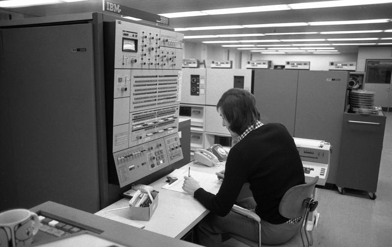
An IBM 360
An IBM System/360 in use at Volkswagen.
German Federal Archives
A third generation computer consisted of a group of large metal boxes. The cabinets were laid out in an air-conditioned machine room and connected with heavy-duty cables under a raised floor. Photographs show machine rooms that were models of tidiness, but in practice a machine room was a busy place, full of boxes of punched cards, magnetic tapes, and stacks of paper for the line printers. They were noisy, with card readers and line printers chattering away and the continuous rush of air-conditioning.
Solid-state components had replaced vacuum tubes, but the logic boards were still large and the central processor was several tall racks of circuit boards with interconnecting cables. Memory used magnetic cores, which were bulky and expensive. In 1968, the price of memory was about $1 per byte.
Most of the boxes in the machine room were peripherals and their controllers. Rotating disks were beginning to come on the market, but most backing store was on open-reel magnetic tape. The tape held nine bits of data in a row across the tape, representing one byte plus a check digital. Early drives wrote 800 rows per inch, but higher densities followed steadily. To sort data that is on magnetic tape requires at least three tape units and most systems had many more. The controllers that connected the tape and disk units to the central processor were imposing pieces of expensive hardware.
The architecture of the IBM 360 supported both scientific computing and data processing. It firmly established the eight-bit byte as the unit of storage for a character and four bytes were organized as a word. Earlier computers had used a variety of word sizes and characters had often been stored as six bits. In the days before virtual memory, memory was organized into 4096 byte modules and I vividly remember the challenges of memory management when writing assembly code programs.
The instruction set was designed to support high level languages, such as Cobol for data processing, and Fortran for scientific work. Arithmetic could be decimal, operating on character strings, or binary, operating on words that could represent either integer or floating point numbers. By using variable length instruction formats, complex operations could be carried out in a single instruction. For example, only one instruction was needed to move a string of characters to another location in memory. Apart from the memory management, I found the assembly code straightforward and easy to program in.

A Fortran coding sheet
Programmers wrote their code on coding sheets. A clerk keyed the program on to punched cards, one card for each line of the program.
Photograph from Wikipedia
In the days before terminals and interactive computing, a programmer wrote the instructions on coding sheets, with one 80-character line for each instruction. The instructions were punched onto punched cards, one card per instruction. A colored job control card was placed at the head of the card deck and another at the end, followed by data cards. The complete deck was placed in a tray and handed to the computer operators. Some time later the programmer would receive a printout with the results of the compilation and the output of any test runs. Computer time was always scarce and one test run per day was considered good service. This placed a premium on checking programs thoroughly before submission as even a simple syntax error could waste a day's run.
Batch processing
Data processing applications used batch processing to automate tasks such as billing, pay roll, stock control, etc. The algorithms resembled the modern "map/reduce" methods that are used to build indexes for Internet search engines. These methods are used when the amount of data is so large relative to the memory of the computer that there is no possibility of holding comprehensive data structures in memory and random access processing would be impossibly slow. Therefore the processing methods use sequential processing. The basic processing steps are sorting and merging, and the computation is done on small groups of records that have the same key.
In earlier years, some data input had used paper tape, but by the late 1960s punched cards were standard. An advantage of punched cards was that an error could be corrected by replacing a card, though it was easy to make further mistakes in doing so. Every computer center had a data preparation staff of young women who punched the transactions onto punched cards in fixed format. The cards were verified by having a second person key the same data. Data preparation was such a boring job that staff turnover was a perpetual problem. The British driving license system, which we developed at English Electric - Leo, was always understaffed in spring before the school year came to an end and the next wave of school leavers could be hired.
The first step in processing a batch of cards was to feed them into a card reader. A "data vet" program checked the cards for syntax errors and wrote the card images onto magnetic tape. This was then sorted so that the records were in the same sequence as the master file.
Records were stored in a master file on magnetic tape and sorted by an identifying number, such as a customer number. Sorting records on magnetic tape by repeated merging was time consuming. The performance depended on the number of tape drives and the amount of memory available. Time was saved by having tape drives that could be read backwards, so that no time was wasted rewinding them.
The master file update program would typically be run at the end of the day. The previous version of the file would be merged with the incoming transactions and an updated version of the master file written on a new magnetic tape. The update programs generated copious output to be printed including business transactions such as bills or checks, management reports, and data errors. This output was written to another tape, which was then sorted by the category of printing, so that the operators could load the various types of paper into the printers as required.
The standard printer was a line printer, usually upper case only. The paper was fan-folded with sprocket holes on the side and was advanced one line at a time. Most manufacturers used drum printers, with a complete set of characters around the drum, but IBM used a chain printer in which the characters were on a moving chain. I never understood how it worked. With either type of printer the actual printing was caused by a flying hammer that pressed the paper against the metal character.
Every part of the operation was prone to failure. Most computer centers halted work for several hours every night for maintenance, but even so hardware and software failures were common. An advantage of batch processing was that the system could write a checkpoint at the end of each batch. If the card reader jammed or a magnetic tape failed, the operators went back to the previous checkpoint, and reloaded the cards or the previous copy of the tape and restarted the job.