Montecarlo Raytracing vs. Raytracing

Montecarlo raytracing let you simulate the light transport in a very accurate (and time-consuming) way.
Here are some of the detail of my two different implementations and images compared to the images obtained by raytracing to show some of the possible effects you can obtain by rendering with Montecarlo techniques.

Implementation using RenderMan

The first of my implementation used Pixar RenderMan shading language.
This language is really powerful and let you implement in a very few line a Montecarlo raytracer.

I implemented a very simple Montecarlo raytracer using a normal Montecarlo sampling and stratified sampling. I also added Next event estimation optimization, that reduces the noise a lot, but I should check better before being sure that the integration is completely correct (the image seems to be). The implementation is straightforward in RenderMan (about 30 total lines of code).

• Pros
• Simplicity - RenderMan is simple and powerful
• Simple comparisons - With BMRT you can directly compare to a two pass renderer
• Extensibility - In the language is very simple to implement different forms of BRDFs and is also simple to implement various kinds of texture that are a pretty powerful modeling technique to add details.
• Scene language - RIB is a very powerful scene language and is also supported by a lot of other libraries and modelers (Rhino, VTK, 3DSMax to name a few).
• (RenderMan is industrial supported)
• Cons
• Speed - Since a RenderMan shader is compiled as a bytecode, other implementation are faster
• Flexibility - It is not possible to implement a path-tracer in the language (at least I don't know how to do).
• File output format - Since the file output format is TIFF (in BMRT), the precision of the saved luminances are too low for a Montecarlo raytracer. I mean that is very very frustrating rendering a test for 3/4 hours and discovering that you have just render a completely black scene! This is probably the unique real good reason for using another implementation. Obviously this can be simply fix by exporting the file in an other format, but I can't do it in BMRT.

Implementation by modifying Rayshade

The feature of this implementation are the same as above with the addition of an option for using pathtracing technique. I also implement a feature for including the rendering of only the direct illumination, that can be helpful if you want to compare results in the images you render.
To spare time, all the option are hardwired in an initialization function in the code. This is not so bad, since I only run the code in debug mode, to check some strange instabilities that sometimes happen (I have no clue why), and since I am only looking for possible bugs somewhere.
Using Rayshade I had a lot of problems, because strange things happens sometimes, and I really don't know why now (I didn't spend so much time in trying to figure out what can be. My idea is that some strange things happens using Rayshade libraries and Microsoft compiler - see below).
I also implemented next event estimation (that is just render the direct illumination contribution in a separated way from the indirect), but I can't really use it because it is pretty unstable. I implemented a "biased" Montecarlo integration and in this way works perfectly, but it is biased, so it is physically wrong.

• Pros
• Flexibility - I can write down a pathtracer.
• File output format - I can save the file in a more precise format - Utah rle or my own SIF (Silly image format) format.
• Speed - As expected, the computer time is less then the BMRT implementation. A reason can be the fact that I am using compiled code, instead of interpreted one.
• Cons
• Simplicity - The language and the libraries are not so powerful as RenderMan (at least I need to write more code to do the same things).
• Compiler incompatibilities - Since Rayshade in partly written in K&R C, it is really hard to integrate C++ classes in the project and compile them. It is also impossible to use a lot of the function in VC IDE, that can compile K&R C, but is really better is you use ANSI C. This is probably to biggest cons at all, since the libraries are really cryptic, and I could not use my own libraries (because they are C++ code, and I cannot include C++ header in K&R C code). The coding standards are strange (see for example the operation on vector, where sometimes you need a pointer, sometimes an object...) and this really slow down the time you have to explore new features.
• Compiler instabilities - I don't know way, but it seems to me that VC++ 5 is pretty unstable if I try to compile the code (there should be no reason way I can't include C++ classes in K&R, but with this particular code, I can't). Partly this can be due to the fact that the code is not ANSI C, so it is not supposed to be supported "in a good way" by the compiler, partly because VC++ 5 is just unstable, probably. I really have no clue for judging this issue, so these are only my hypothesis.
• Scene language - This language is really non powerful! This make me spend a lot of frustrating time to model two simple cubes (there is no primitive), or a very simple closed cylinder (you need explicitly add the cap). As far as I know this scene language is only supported by this program.

Timing

Since I am evaluating the time of the algorithm using the number of rays casted (the execution of the rendering function is linear with respect to them), I can simply use the formulas for calculating how many ray I cast to evaluate the running time.
For the raytracing implementation, the running time is res * (1 + light_res), where res is the resolution of the rendered image, and light_res, is the number of sampling used to approximate the light source.
For the pathtracing approach, the number of rays casted is res * (1 + res_theta * res_phi * depth), where res_theta is the number of subdivision for the angle theta,  phi for the angle phi, and depth for the recursion depth. I normally take res_theta = res_phi / 4.
For the Montecarlo approach, the number of rays casted is res * (1 + (res_theta * res_phi) ^ depth).
The code runs in about 50 minutes for a pathtracing with depth = 8, res_phi = 16 and res_theta = 4.
 

Image comparison

To compare the speed of the various algorithm used, I decided to compare just the number of total ray casted.
This should be a good measure if you want to compare the quality vs. time ratio between the various algorithm used. It is also better than comparing the processor time since I always run the code in debug mode from the IDE, while I am working on other programs, so this measure is not good enough.

Raytracing images

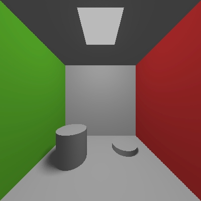
I firstly render some images using raytracing. The scene a modified version of the Cornell box rendered using the implementation based on Rayshade.
As expected, you loose interreflection, that is to say that raytracing is ok as far as the contribution of indirect light is small. We can also say that it is ok as far as the gradient diffuse light is really small in the region we want to render. The value of ambient light I choose is just a trial value. You should normally try to match it with the scene you want to render (especially if you are working in a interactive local illumination environment to model the scene).
The soft shadows can be obtained using jittered sampling of the area light source in the ceiling, so as argued before, this is not a problem for raytracing (at least you can simulate them such that the scene looks "reasonable").
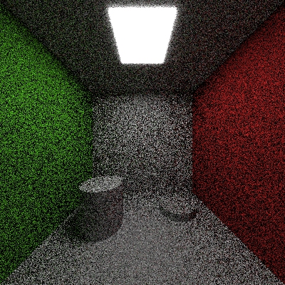
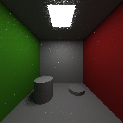
Here are three images rendered using different samplings for the area light. As expected the noise is reduced a lot from the first to the last image simply by taking more sample on the light source.
 

Pathtracing images

As it can be see from the images, the noise is really a lot. Even by changing the depth of the recursion for raytracing, the noise seems to practically not be so different from before, even if the rendering time grows almost linearly with the depth (see above).
I also tried to render a high resolution image and using some image processing program to apply some filters, but, as expected, this is practically unuseful since the noise is too high.
Just by playing with the gamma and exposure value in glimage, it is clear that the lack of the direct illumination contribution is the main reason for such a noise at low number of sampling per pixel (this is pretty obvious physically, but having a proof is always good).
See below for same images.

Pathtracing images using stratified sampling

Stratified vs. non-stratified sampling

As expected, this very simple modification reduce the noise quite a bit, Chile maintaining the same rendering time.
Here are two images rendered for depth = 2, res_phi = 16 and res_theta = 4.
As can be seen in the central part of the floor, and on the central part of the walls, the noise is clearly reduced even if I am using the same number of points.
 

	Non-stratified sampling depth = 2 res_theta = 4 res_phi = 16
	Stratified sampling depth = 2 res_theta = 4 res_phi = 16

Variation with resolution of the stratified grid

As can be expected by the geometry of the scene, direct illumination plays a very important role. This is due to the fact that a lot of the surfaces in the scene are illuminated by direct lighting, this is the most important contribution to the illumination of these surfaces. So to reduce drastically the noise in this areas it is really important to raise as much as possible the resolution of the stratified sampling grid to raise the probability to hit the light.
Here are three images rendered using pathtracing and stratified sampling, with different grids for theta and phi.
 

	depth = 2 res_theta = 4 res_phi = 16
	depth = 2 res_theta = 8 res_phi = 32
	depth = 2 res_theta = 16 res_phi = 64

Variation with the depth

As before, the depth plays not a so important role on reducing the noise, since it is important only for indirect illumination. Since also the contribution of a random walk is greater than zero if it hit the light source in the scene, than it is clear that also the probability to have a contribution for indirect illumination does not converge very fast and the noise for the indirect contribution is very large.
 

	depth = 2 res_theta = 4 res_phi = 16
	depth = 4 res_theta = 4 res_phi = 16
	depth = 8 res_theta = 4 res_phi = 16

Montecarlo raytracing

Since the time to render a Montecarlo image is exponential with the recursion depth, the quality/speed ratio is not very good. To be useful you have to use a very low depth. Since as shown above the real important thing is raising the res_phi and res_theta as much as possible, the depth used is really really low. In a diffuse environment where direct light plays an important role, like here, this is not a so bad. This is because in every case the most important contribution to a lot of the surface area in the picture is due to direct lighting, so trying to getting its contribution is the most important thing normally.
But as can be clearly see by the comparison below, the area with indirect illumination (ceiling and cylinders in shadow), have a clearly better look now than using a pathtracing.
 

	Montecarlo depth = 2 res_theta = 4 res_phi = 16
	Pathtracing depth = 2 res_theta = 4 res_phi = 16

Next event estimation optimization (implementation using angles)

I implemented also next event estimation, but it seems to crash to program. So I implemented it in a biased way. In this way the integrals are not estimated correctly since I am biasing the random distribution of casted rays, but it is good to estimate the convergence of the code. As expected the convergence is made very fast in this way.
Here is an image obtained in this way compared to the same one without the implementation.

Next event estimation optimization (implementation using areas)

Since the code that uses the angle implementation was biased (in the sense that the non-biased one crashes everything), I decided to implement a NEE using area integral instead of angles.
This implementation runs ok, but I decided to leave the other images such that a comparison can be made. It is interesting (at least for me), to see what does it means to bias the result of a Montecarlo integration.
All the images in the table below are obtained at the same resolution, but it is clear that the next event estimation one converges faster.

	Next event estimation depth = 2 res_theta = 4 res_phi = 16 light sampling = 2x2 jittered
	Pathtracing depth = 2 res_theta = 4 res_phi = 16
	Biased next event estimation depth = 2 res_theta = 4 res_phi = 16 light sampling = 4x4 jittered