In this project we are asked to implement Harris corner detection, Multiscale Oriented Patches feature desciption (MOPS), a simple window feature descriptor, and an original feature descriptor.
One of the challenges I found when working on this project was that the feature detection algorithms asked for a set threshold to determine whether a pixel was a feature or not. The selection of this threshold proved difficult, especially on the bikes and the leuven data sets. In the bikes set, the images are progressively more out of focus, and a theshold that provides a manageable number of features in the first image provides zero features in the last image. For the leuven data set, the images are progressively darker, with similar (though not quite so drastic) results.
To mitigate these problems, I normalize the calculated Harris image such that the mean is 0.5 and the variance is 0.2. This allows me to set a threshold that should return roughly the same number of features across all images. However, such an approach could potentially return a large number of weak features in some cases (a photograph of a blank featureless wall, for example). In the given images, where the reason for few features was underexposure or bad focus, this approach works fine.
I implemented the MOPS descriptor as described in class: select a 40x40 window around the feature, oriented to the largest eigenvector of the Harris matrix at that feature (interpolating to find the value at that location), subsample to 8x8 pixels, and normalize using the mean and variance of the pixels. For pixels that fall outside of the original image, I assume the pixel values are 0.5 (gray).
Here we simply select the region around the feature, and these pixel values become the descriptor. No other operations are performed.
My custom feature descriptor focuses on the image gradient. Like the MOPS descriptor, it samples an oriented 41x41 patch around the feature (this time oriented using the smoothed gradient at the feature location). Within this patch, it looks at 5x5 sub-patches.
In each of these sub-patches, the gradient is calculated using a finite difference at the 25 pixels. The mean and variance of the heading is calculated (with each pixels gradient magnitude used as its weight, with the sum of the weights normalized to 1). In addition, the sum of gradient magnitudes is calculated.
There are 64 such 5x5 pixel regions. The mean and variance of the gradient angle is saved for each region. Because these values are computed using the normalized gradient magnitudes, these values will be invariant to intensity changes in the original image, and make up 128 elements of the descriptor.
We also have the sum of gradient magnitudes for each of the 64 sub-patches. These are normalized by their mean and variance to ensure invariance to brightness changes and stored as elements of the descriptor.
In addition, I wanted to capture an element a features similarity to the other features in the scene as a description of that feature. I calculate the mean and variance of the angle of all of the features in the feature set, and compute the probability of a given features angle having been sampled for a normal distribution of that mean and variance as a descriptor.
This makes a total of 193 elements of four different types in the descriptor vector. Each type gets its own weight (for example, the probability term ranges between 0 and 1 and makes up a single element – for it to have any impact on matching it must be weighted higher than the other terms).
One challenge in this detector is when comparing two different angles to each other, care must be taken to recognize that, for example, -.9*PI and .9*PI are very close to each other, and don't average to 0. This is accomplished in a series of checks where applicable in the descriptor code.
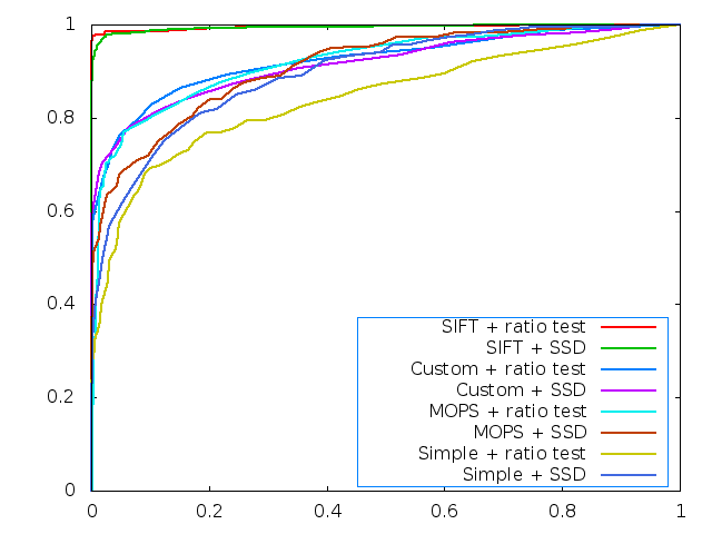
For the Yosemite pictures, we calculate the features using the three different descriptors, and use the built in functions to calculate the ROC curves for each descriptor, for both direct matching and ratio test matching.
As we can see from the image, the SIFT features far outperform all of the features implemented in the project. Of the rest, the custom descriptor performs the best by a small margin for lower matching thresholds, and is eventually caught by the MOPS descriptor at higher thresholds.
Also of interest is that the simple feature descriptor performs very well for this image. Given that the two images are essentially translations of each other with no additional transformations, this is as expected.
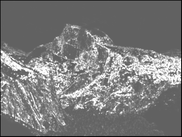
This image shows the Harris values of the image. The Harris values have been scaled as described above, accounting for the brightness of this image.
The same curves were calculated for the first two images in the graffiti data set. This is a much more challenging data set, as the camera position and orientation change between images. The ROC curves from the three descriptors are:
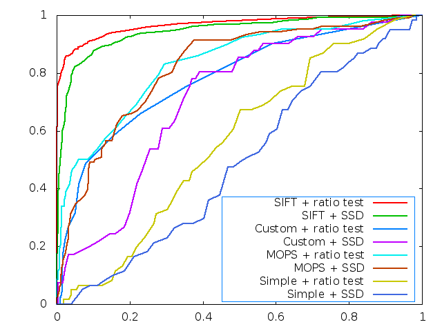
Due to the increased difficulty, we see that the simple descriptor fails completely. The custom descriptor (with a ratio test used for matching) performs closely with the MOPS descriptor. As before, the SIFT descriptor is far better than any implemented in this project.
The following table reports the AUC scores for the benchmark data sets:
|
|
Graffiti |
Wall |
Bike |
Leuven |
|
Simple Descriptor |
0.526 |
0.544 |
0.531 |
0.540 |
|
MOPS |
0.579 |
0.639 |
0.674 |
0.663 |
|
Custom Descriptor |
0.566 |
0.568 |
0.601 |
0.583 |
In general, the custom descriptor performs somewhere between MOPS and the simple descriptor. I believe that with much time spent tuning the weights in the custom descriptor, performance could be improved. Also, the feature matching would need to be modified to look at the smallest possible distance between angles rather than the absolute distance (i.e. .9*PI and -.9*PI are 0.2*PI apart from each other, not 1.8*pi).
All the descriptors work reasonably well with sets where the transformation between the pictures is a simple translation. The simple descriptor does not handle any other transformations without breaking. Both the MOPS and the custom detector are designed to also handle changes in brightness (both offsets and scaling) and rotations as well as simple translations. The custom descriptor does not match features as reliably as the MOPS descriptor, even though it uses a larger number of descriptors.
Because the custom descriptor incorporates the orientation of all of the features in the set, the presence of an object in one picture and not the other with enough features to significantly alter the distribution of feature orientations can cause major changes to the descriptors of other features in the image.
I ran the feature matching algorithm on some pictures I took last Fall at the 2010 Vintage Grand Prix at Watkins Glen. I compare two photographs of the same corner at different times (with different cars in the foreground), several pictures of the several-time LeMans winning Audi R10 to see if any of the algorithms would be able to recognize the car from different angles and distances, and a set of pictures of a Corvette after a loss of control.
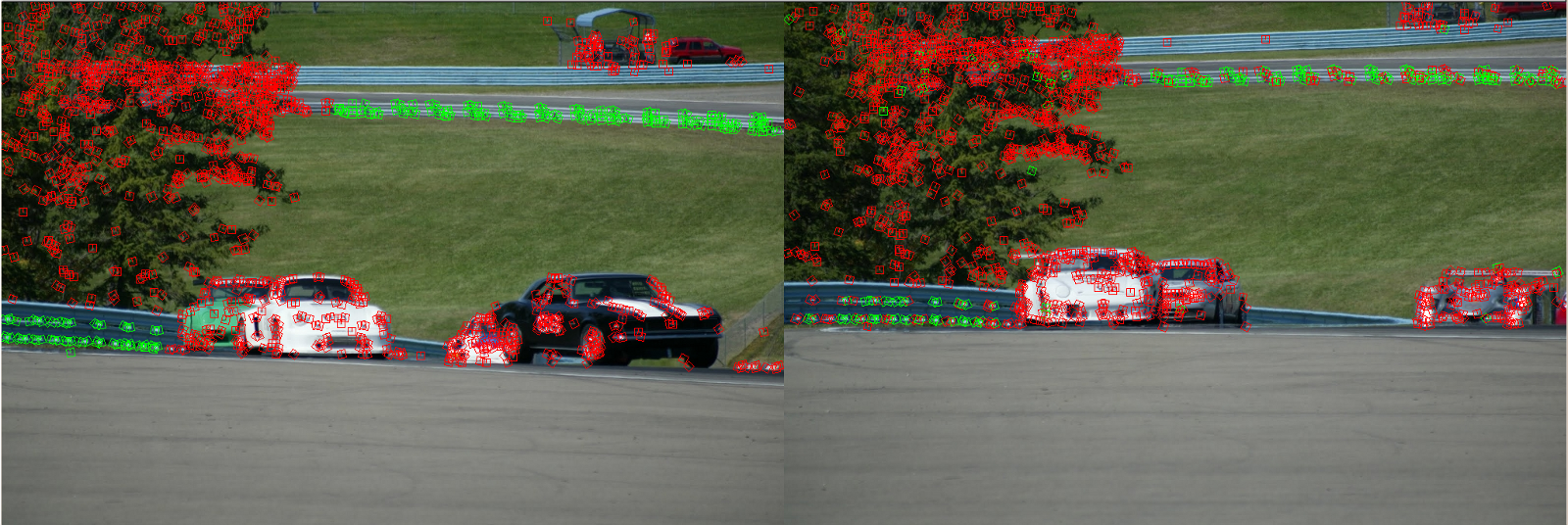
This image shows two selected groups of features matched across two images with different foregrounds.
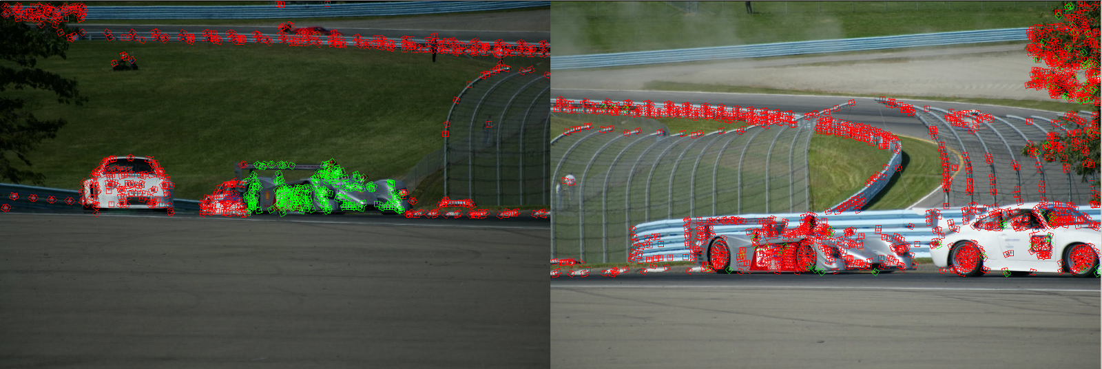
This image shows that even with a relatively slight change in perspective, almost no features are matched between the different pictures of the Audi R10. This was true for both the MOPS descriptor and the custom descriptor.
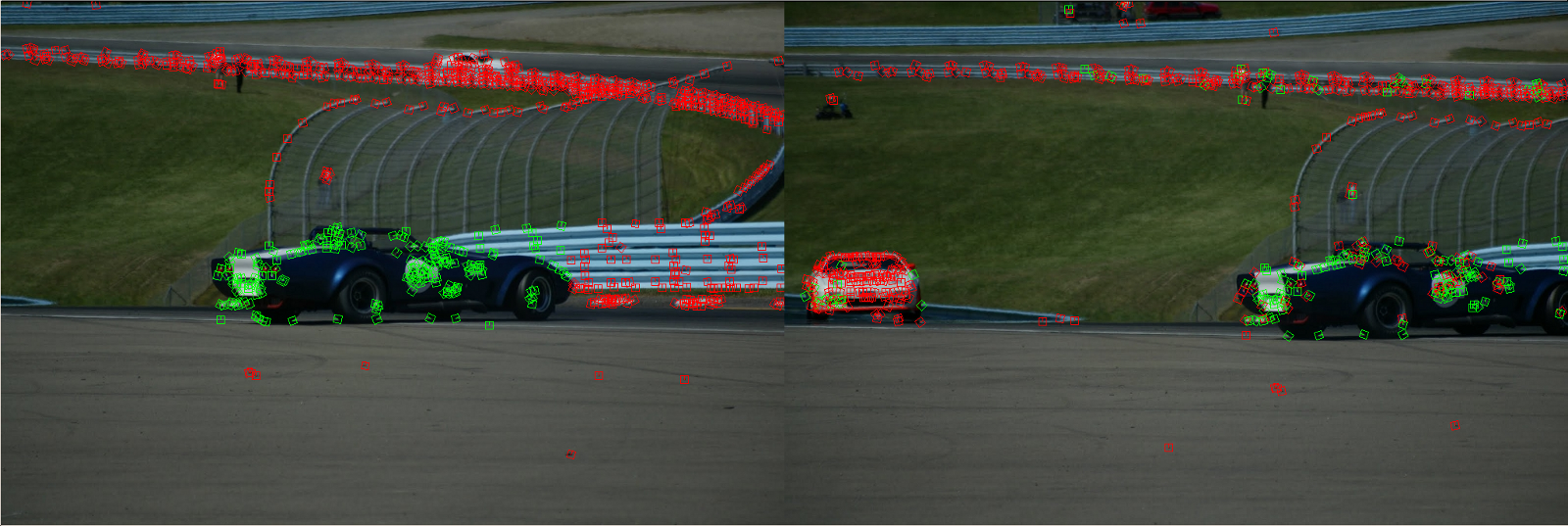
Here we see very strong matches between the two images of the spun Corvette.
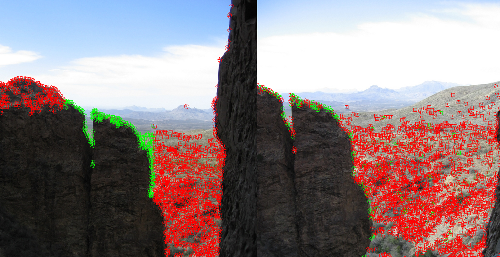
I also ran my matching algorithm on a pair of images I took from the end of the Window trail in Big Bend National Park in West Texas. Again, it appears that the selected features are matched with a reasonable ratio of true positives to false positives.
Both the MOPS and the custom descriptor (with some tuning) work reasonably well for many transformations between images. However, for anything that changes the scale or perspective, both descriptors fall apart and something better will be required.