CS6670 Project 1: Feature Detection and Matching

Bingxin Xu

bx38@cornell.edu

1. Feature Detection

In this step, we identified the points of interest in the image using the Harris corner detection method.  The steps are as follows, for each point in the image, consider a window of pixels around that point.  Compute the Harris matrix H for that point, defined as

where the summation is over all pixels p in the window.  The weights should be chosen to be circularly symmetric (for rotation invariance).  In our case, we use a 7x7 Gaussian mask.

Compute the corner strength function in order to find interest points

The interest point is the local maximum in a 5x5 window.

The orientation of the feature is obtained by calculating the gradient at that point. The mask matrix is as simple as:

M_dx =   ,  M_dy =

And get the orientation as:

θ = atan(dy/dx)

by doing this, we managed to avoid calculating eigenvalues of every single H matrix.

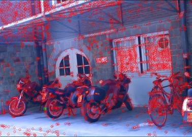
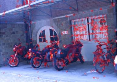
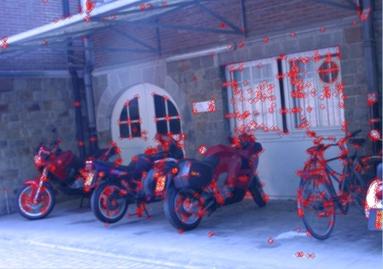
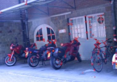
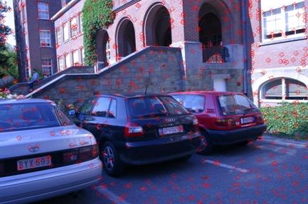
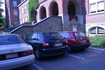
Examples:   threshold = 0.01 for Harris value

Below list all the example images

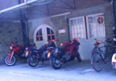
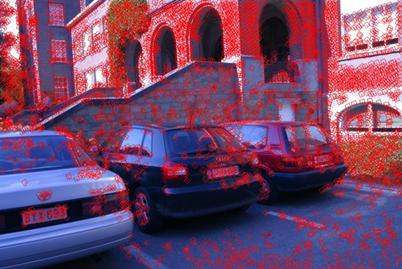
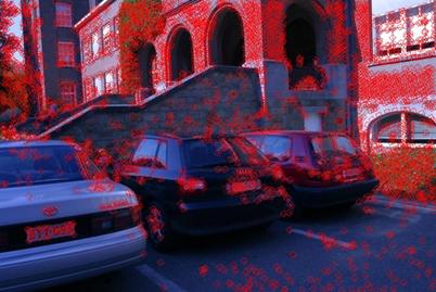
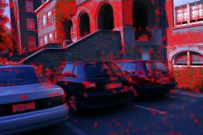
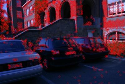
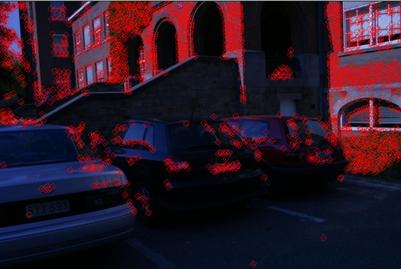
And a personal example to test scale invariance:

2. Feature Description

2. 1 Simple descriptor

This descriptor obtains a 5x5 square window of near neighbors centered at the feature point without orientation.

Advantage:

It is translation invariant. Illumination invariance is obtained by normalizing the descriptor.

Disadvantage:

Nothing to do with scale.

2. 2 MOPS descriptor

The descriptor is formed by first obtaining a 41x41 square window of near neighbors centered at the feature point with orientation, and then down sampling to a 8x8 square window. And then normalize the descriptor.

Advantage:

It is translation invariant. Illumination invariance is obtained by normalizing the descriptor. Orientation included.

Disadvantage:

Nothing to do with scale.

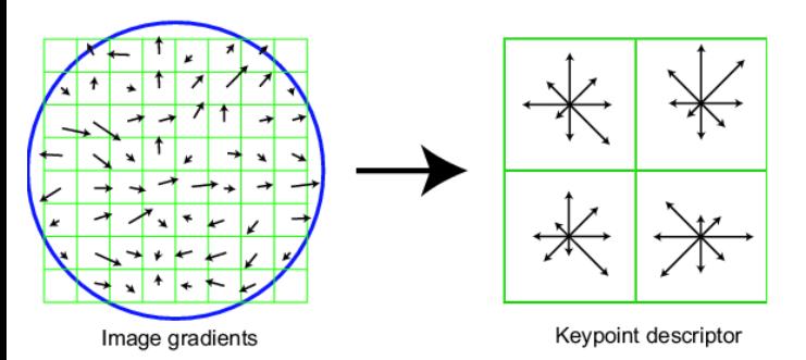
2. 3 Customed Version of SIFT

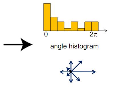
Here I design my costumed descriptor as a lite version of SIFT. Instead of obtaining grayscale intensity near the feature point, in this descriptor I obtain histogram of gradient near the feature point. I firstly calculate a 16x16 square window of near neighbors centered at the feature point with orientation. And then divide the window into 4x4 grid, and calculate the histogram of gradient angle in every 4x4 grid. Then we have 16 histogram in a 16x16 big window. Set the mode of histogram as π/4. Thus for every feature point, we have an 8x16=128 dimensional vector as descriptor.

A simple demo is as below:

Advantage:

Translation and illumination changes can be handled very well. Orientation included. Scale invariant.

Disadvantage:

Apparent my costumed version of SIFT is very good (see below ROC comparison). It is comparable to MOPS. The reason that performance is not dominantly improved is the size of window. I used 16x16 to plot histogram. Maybe a bigger window is suggested…

3. Feature Matching

3. 1 Discussion of matching performance

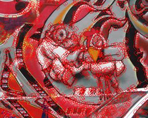
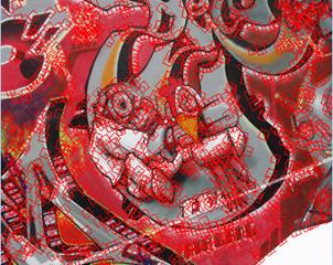
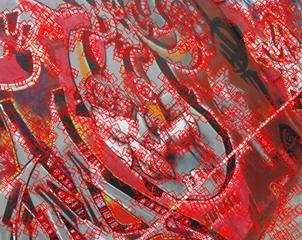
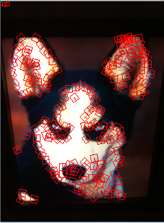
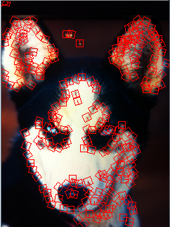
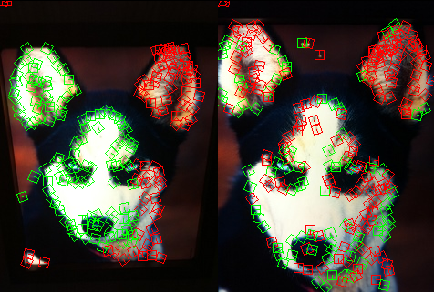
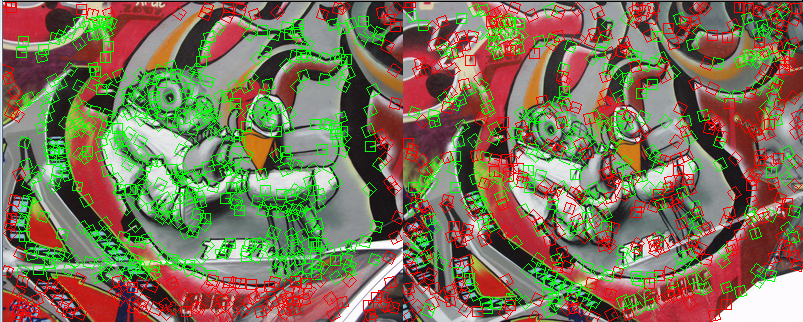
Several examples are shown below. We use the costumed descriptor and SSD matching. 

For the first example of dog, note that the features of right ear was not selected, and the matching works pretty good.

3. 2 ROC curves

The ROC curves for the Yosmite and graf image are given below. I don’t know why we get a strange curve for the Pyramid descriptor by SSD matching algorithm, I guess one possible explanation could be pyramid descriptor is not very valid since it takes a pyramid structure as the descriptor, there could have some error during the blurring and downsampling process, or there are some bugs within my code. Put this aside, all the rest curves seem reasonable. From the figures, we can see that SIFT gives the best performance, MOPS descriptor gets the second place, then the simple descriptor and finally the Pyramid descriptor.

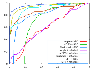
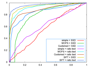
graf                                                                                   Yosemite

The AUC for the above two sets of images is listed as follows:    

	Graf	Yosemite
Simple + SSD	0.595137	0.566606
MOPS + SSD	0.702675	0.790221
Custom + SSD	0.814013	0.845468
Simple + Ratio	0.599196	0.620979
MOPS + Ratio	0.914771	0.933490
Custom + Ratio	0.866368	0.888095

3. 3 AUC report

Below is the average AUC report for the feature detecting and matching code for the four benchmark set: graf, leuven, bikes and wall. Here the match type is chosen to be the ratio matching algorithm. The data structure in the following table is Average error \ Average AUC.

Note: The program reports error when I applied to graf dataset… Can’t figure out the reason.

SSD:

Average Error:

	Simple 5x5	MOPS	Custom
Graf
Bikes	404.173733		405.467059
Leuven	255.379574		311.577155
Wall	354.595455		355.592734

Average AUC:

	Simple 5x5	MOPS	Custom
Graf
Bikes	0.523970		0.603305
Leuven	0.580441		0.568675
Wall	0.583874		0.604059

Ratio:

Average Error:

	Simple 5x5	MOPS	Custom
Graf
Bikes	404.173733		405.467059
Leuven	255.379574		311.577155
Wall	354.595455		355.592734

Average AUC:

	Simple 5x5	MOPS	Custom
Graf
Bikes	0.545173		0.593358
leuven	0.609033		0.648450
Wall	0.584888		0.625035

4. Summary & discussion

1. In simply words, we implemented the feature detection, feature description, feature matching in this project. We use our program to test several benchmark dataset and our own images. In my opinion, the results look good.

2. The discussion of strength and weakness of every descriptor is included in the section 2.

3. One thing need to mention is the features near boundary. Since we use a window centered at feature, the window may exceed the boundary of image when the feature point is near the boundary. In this case, we are supposed to erase the feature point from the list. While the problem is, the program is too large. If I simply erase one feature point, it results in error at some other place in the program. Given condition that the feature file contains lots of information like feature ID and feature number, the bug is understandable.

So what I did is assign ZERO value to the f.data of feature points that exceeds boundary. It has significant drawback that the program still try to find matching for features which actually has no descriptor. This is one of the most important reasons that reduces the performance. I know the problem but didn’t have time to debug it.

4. A weakness of such feature detection is that we treat every feature as a local point, which lost the global relevance between the feature points. When we do the matching, I would suggest match all the feature points as an entire point set. Maybe we can introduce the Interactive-Closest-Points (which can be integrated with KD-Tree). But if we do this, we basically lost the feature descriptor… I’m still thinking of a better method to integrate the ICP algorithm. A simple experiment is shown below in the extra credits.

Extra Credits:

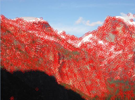
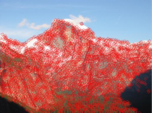
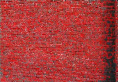
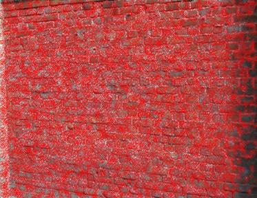
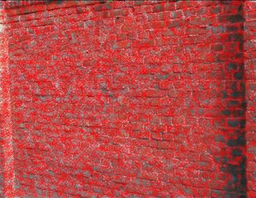
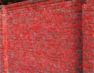
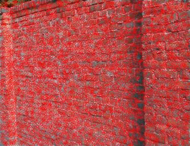
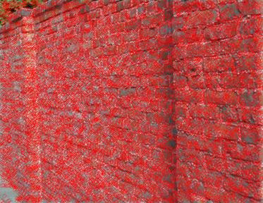
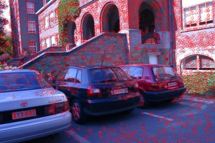
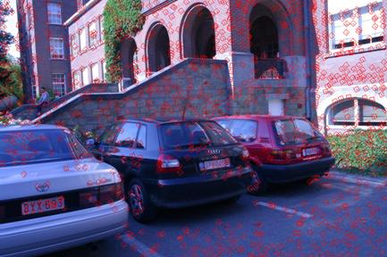
1. Adaptive Non-Maximal Suppression

 For better matching and recognition in databases, it is good to limit the number of features in each image. I set this threshold to several values by observing performance on provided datasets. One way to truncate features is to just pick first 1000 features in order of their harris function value. But this gives a bad distribution of the features over the image. Instead, I implemented MOPS which adaptively chooses features based on their proximity to each other thus giving a well distributed set of features over the image. This comparison of feature distribution can be seen in the following figure.

Experiments:

                                          i =2000                                                                                               i =1000

                                          i =500                                                                                                   i =100

2. Interactive Closest Points

Iterative Closest Point (ICP) is an algorithm employed to minimize the difference between two clouds of points. ICP is often used to reconstruct 2D or 3D surfaces from different scans. It gives a transformation matrix from testing data to training data in order to achieve the least difference.

The algorithm is conceptually simple and is commonly used in real-time. It iteratively revises the transformation (translation, rotation) needed to minimize the distance between the points of two raw scans.

Inputs: points from two raw scans, initial estimation of the transformation, criteria for stopping the iteration.

Output: refined transformation.

Essentially the algorithm steps are :

1. Associate points by the nearest neighbor criteria.

2. Estimate transformation parameters using a mean square cost function.

3. Transform the points using the estimated parameters.

4. Iterate (re-associate the points and so on).

Ref: http://www.cs.princeton.edu/~smr/papers/icpstability.pdf

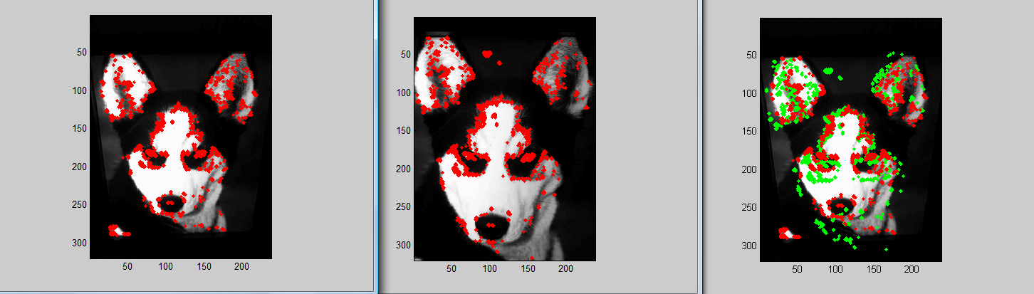
Left figure shows img1 and feature points of img1.

Middle figure shows img2 and feature points of img2.

Right figure shows the projected feature points (in green) obtained from img2 compared to the original feature points(in red) of img1.

Reference

[1] Cook, J.;   Chandran, V.;   Sridharan, S.;   Fookes, C.  “Face recognition from 3D data using Iterative Closest Point algorithm and Gaussian mixture models”, IEEEX

[2] M. Sun, G. Bradsky, B. Xu, and S. Savarese, "Depth-Encoded Hough Voting for Joint Object Detection and Shape Recovery", Proc. of European Conference of Computer Vision (ECCV), 2010

 [3] K. Mikolajczyk and C. Schmid, "Indexing based on scale invariant interest points", International Conference on Computer Vision 2001, pp 525-531

[4] K. Mikolajczyk and C. Schmid, "Scale & Affine interest point detectors", International Journal of Computer Vision 60(1), 63-86, 2004

[5] David G.Lowe, "Distinctive image features from scale-invariant keypoints", International Journal of Computer Vision, 60, 2 (2004), pp. 91 - 110

[6] M.Brown, R. Szeliski and S. Winder, "Multi-Image using multi-scale oriented patches", International Conference on Computer Vision and Pattern Recognition 2005, pages 510 - 517