CS 6670 Project 1
Akram Helou

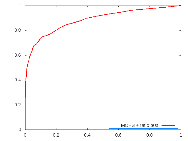
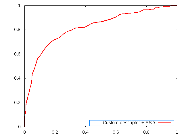
I have experimented with two approaches for my feature descriptor. The approach which the results are drawn from involves a couple modifications of the simple MOPS descriptors. The first modification is changing the final windows size from 8*8 to 9*9. My simple MOPS implementation indicates that a 9*9 window is more effective than a 8*8 window based on marginal improvements in average error and average AUC on the benchmark datasets. This modification was done to increase the specificty of the descriptor vector.
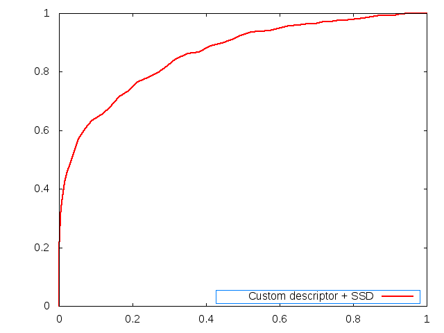
The second modification is normalizing the final descriptor vector by subtracting the mean and dividing my the standard deviation. Again, this resulted in marginal improvements in average error and average AUC on the benchmark datasets. This modification was done to make the descriptor invariant to lighting conditions.
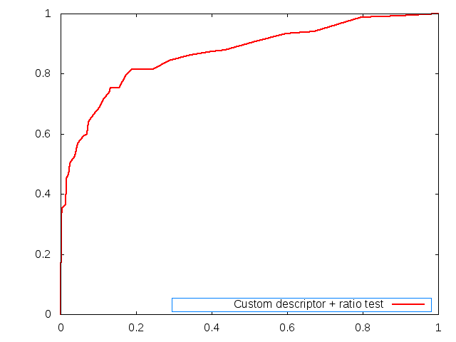
Therefore, the strengths of this mofication is the increase in descriptor specifity and invariance to lighting. The weaknesses are that is not invariant to scale.
 
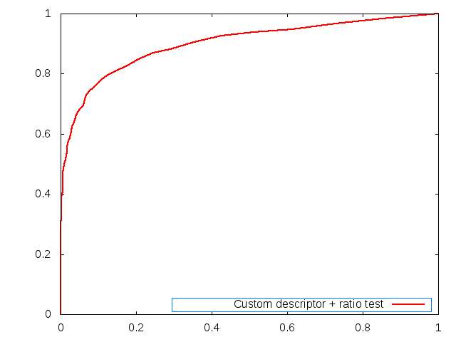
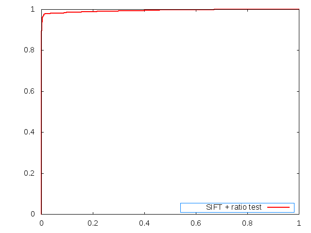
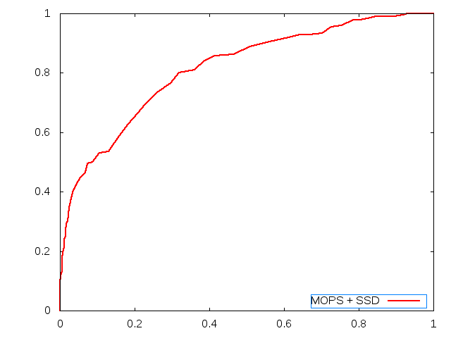
In the second approach (implemented in features_debug.cpp) I attempted to combine ideas from the SIFT feature descriptor with a simple MOPS feature descriptor. This was done by appending to the original MOPS descriptor vector the orientations of the largest gradient values around the location of the feature pixel. I took the top N (for various values ranging from 10 to 1000) gradient orientations and subtracted the gradient orientation of the feature location. I then averaged every M (for values ranging from 10 to 15) normalized gradient orientations to get my final additional descriptors. 
While the average AUC was higher than the first approach on the benchmark dataset, the average pixel error was significantly larger. This indicates that adding these orientations descriptors made every feature too unique to be matched to a similar feature in a different image. Therefore, the weakness of this approach is that I lost the orientation invariance and other invariance possessed by the simple MOPS descriptor. This approach was motivated by the hope of combining the strengths of MOPS (simplicity) and SIFT (performance).

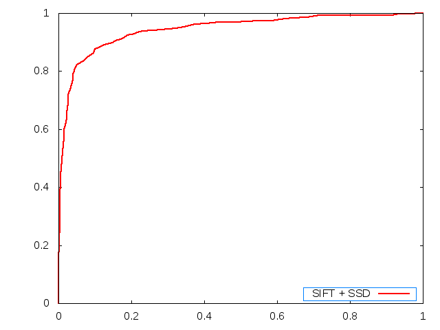
Yosemite ROC data set:










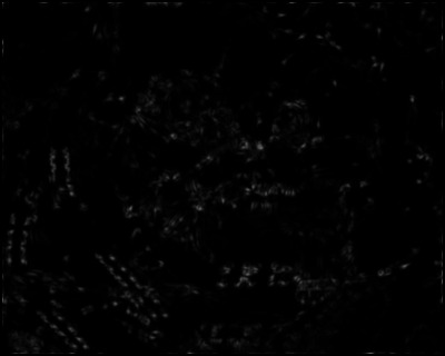
This is the harris.tga image for img1 in teh ROC yosemite dataset
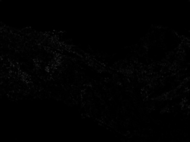yosemite_harris.jpg

Graf ROC dataset:









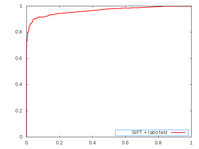
This is the harris.tga image for img1 in teh ROC graf dataset



Benchmark dataset results:

Graf:
average error: 248.843472 pixels
average AUC: 0.605402

Leuven:
average error: 307.990606 pixels
average AUC: 0.616173

Bikes:
average error: 286.186716 pixels
average AUC: 0.639851

Wall:
average error: 262.414206 pixels
average AUC: 0.621211

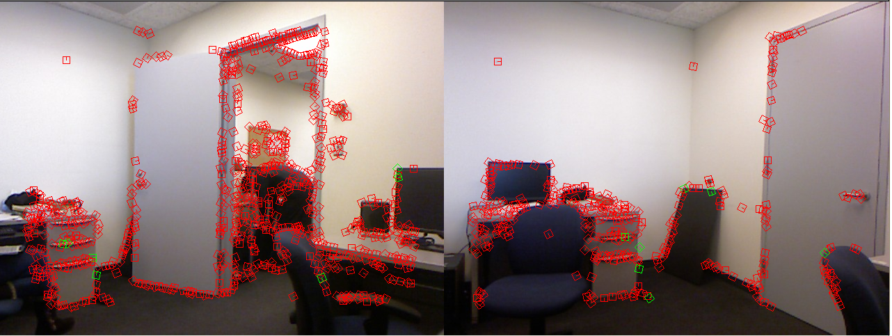
Results for images I took:

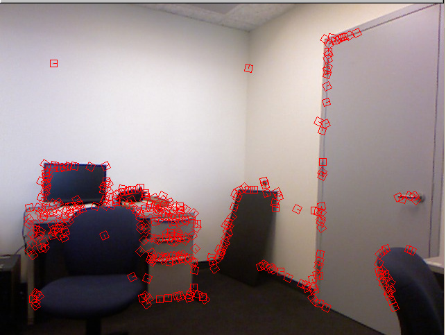
Image 1. These are the Harris corner features with my custom descriptor used.


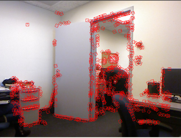
Image 2. These are the Harris corner features with my custom descriptor used.



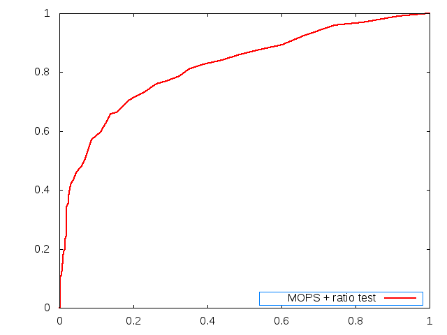
Matches for some features are shown in green. The ratio SSD measure is used for matching.