Project Design Description

My Custom Feature Descriptor

My custom feature detector is built in the following steps:

1) Compute a grayscale image out of the target RGB image, and compute the direction of the image gradient vector at each pixel (The direction is described in angle theta, where 0<=theta<2*PI)

2) Take four 5-by-5 windows around an interesting feature point, in this case a corner detected by the Harris operator. If the interesting point’s coordinate is (x, y), then the coordinate of the upper-left corner of each window will be (x-4, y-4), (x, y-4), (x-4, y), (x, y).

3) For each window, set up an integer array with 8 entries, and initialize each entry to be zero. Now for each of the 25 pixels covered in this window, if the direction, theta, of the gradient vector is in the range [PI/4*i, PI/4*(i+1) ), then increment the i-th entry of the integer array by one. This effectively partitions the possible values of theta into eight bins. The integer array is used to count how many theta falls in a particular bin. Output this integer array.

4) Combine the four integer arrays output from the four windows to form a 32-dimensional vector. This is my custom feature descriptor.

 

Other Design Choicse

I used a 5-by-5 gaussian to weigh each direvative value when computing the Harris values because using a larger gaussian might blur the locality of interesting points, while a smaller gaussian might not be as effective as a 5-by-5 gaussian.

When computing the MOPS descriptor I used a 5-by-5 gaussian to blur the image and then down sample it because a larger gaussian might blur so much that we lose local information, while a small gaussian will make the quality of the downsampled image look really bad. Some early experiments also show that a 5-by-5 gaussian out performs a 3-by-3 or a 7-by-7 gaussian in feature matching.

When computing the Harris value and the MOPS descriptor, I didn’t compute the harris values and the descriptor for pixels that are less than 3 pixel distances to either edge of the image, because otherwise the gaussian filter will have to deal with unknown pixel values, which adds more complexity and a bigger chance of getting into certain errors. Discarding these values won’t really affect anything since most interesting points are not near the edge of the image anyhow.

I implemented the custom descriptor in the way described above because I was curious to see how this descriptor, which is analogus to SIFT except that it uses gradient directions instead of edge directions, would perform against MOPS.

 

 

 

 

 

 

 

Performance

ROC Curve for Yosemite:                                                       ROC Curve for graf:

 

 

 

 

 

 

 

 

 

 

 

 

AUC Values for /yosemite and /graf:

 

 

 

 

 

 

 

 

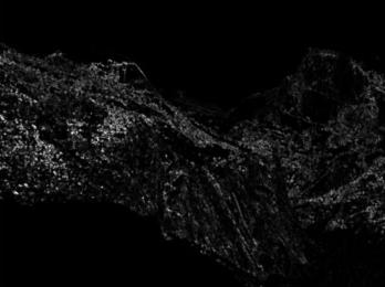
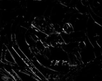
Harris Image for Yosemite1.jpg in yosemite/                           Harris Image for img1.ppm in /graf:

 

 

 

 

 

 

 

 

 

 

 

 

 

 

 

AUC Values for the Four Benchmarks

 

 

 

 

 

 

 

 

 

 

 

 

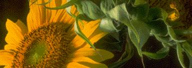
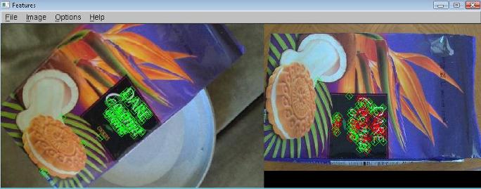
I also tried this project on a pair of images taken at home. The following shows the matching features between these two images. As can be seen, the feature detection and feature matching algorithms works pretty well on this test image because most of the matched features are correct.

 

 

 

 

 

 

 

 

 

 

 

 

 

 

 

 

 

Performance Analysis, Strengthes & Weaknesses

From the above results, we can see that my simplied SIFT feature descriptor doesn’t really work very well in general compared to MOPS, which doesn’t perform as good as SIFT feature descriptor. So using edge directions out performs using image gradient directions by a lot (my custom feature is gradient directions instead of edge directions). But this custom descriptor is better than the simple descriptor in general.

In general, MOPS is the best amongst the three feature descriptors, although there’re a few cases in which MOPS doesn’t perform as good as the other, which is pretty interesting, and should be further investigated.

In general, the ratio distance is better than SSD distance, as can be shown from the AUC values between these two matching algorithms, although there’re a few cases in which SSD matching is better than the ratio distance matching.

The three feature descriptors works much better with the yosemite benchmark than with other benchmarks probably because the two images in the yosemite benchmark doesn’t have too much transformations involved compare to other images, so all together, these three feature descriptors probably won’t work very well in situations where a lot of transformations have occurred in between two images.

 

 

Extra Credit Item

I implemented a simpified version of the Locality-sensitive hashing algorithm. This is implemented in the function LSHMatchFeatures(...) inside features.cpp. To use this feature matching algorithm, simply set matchType to 3 (1 is for SSD, 2 is for ratio test).