CS4670/5670: Computer Vision, Spring 2019
Project 2: Feature Detection and Matching

Brief
- Assigned: Monday, February 18, 2019
- Code Due:
Monday, March 4, 2019 (by 11:59 PM)Wednesday, March 6, 2019 (by 11:59PM) (turn in via CMS) - Report Due:
Wednesday, March 6, 2019 (by 11:59 PM)Friday, March 8, 2019 (by 11:59PM) (turn in via CMS) - Teams: The code and report must be done in groups of 2 students.
Synopsis
The goal of feature detection and matching is to identify a pairing between a point in one image and a corresponding point in another image. These correspondences can then be used to stitch multiple images together into a panorama.
In this project, you will write code to detect discriminating features (which are reasonably invariant to translation, rotation, and illumination) in an image and find the best matching features in another image.
To help you visualize the results and debug your program, we provide a user interface that displays detected features and best matches in another image. We also provide an example ORB feature detector, a popular technique in the vision community, for comparison.
Description
The project has three parts: feature detection, feature description, and feature matching.
1. Feature detection
In this step, you will identify points of interest in the image using the Harris corner detection method. The steps are as follows (see the lecture slides/readings for more details). For each point in the image, consider a window of pixels around that point. Compute the Harris matrix H for (the window around) that point, defined as

where the summation is over all pixels p in the
window.  is the x derivative of the image at point p, the notation is similar for the y derivative. You should use the 3x3 Sobel operator to compute the x, y derivatives (extrapolate pixels outside the image with reflection). The weights
  should
be circularly symmetric (for rotation invariance) - use a 5x5 Gaussian mask with 0.5 sigma (or you may set Gaussian mask values more than 4 sigma from the mean to zero. This is within tolerance.). Use reflection for gradient values outside of the image range. Note that H is a 2x2 matrix.
should
be circularly symmetric (for rotation invariance) - use a 5x5 Gaussian mask with 0.5 sigma (or you may set Gaussian mask values more than 4 sigma from the mean to zero. This is within tolerance.). Use reflection for gradient values outside of the image range. Note that H is a 2x2 matrix.
Then use H to compute the corner strength function, c(H), at every pixel.

We will also need the orientation in degrees at every pixel. Compute the approximate orientation as the angle of the gradient. The zero angle points to the right and positive angles are counter-clockwise. Note: do not compute the orientation by eigen analysis of the structure tensor.
We will select the strongest keypoints (according to c(H)) which are local maxima in a 7x7 neighborhood.
2. Feature description
Now that you have identified points of interest, the next step is to come up with a descriptor for the feature centered at each interest point. This descriptor will be the representation you use to compare features in different images to see if they match.
You will implement two descriptors for this project. For starters, you will implement a simple descriptor which is the pixel intensity values in the 5x5 neighborhood. This should be easy to implement and should work well when the images you are comparing are related by a translation.
Second, you will implement a simplified version of the MOPS descriptor. You will compute an 8x8 oriented patch sub-sampled from a 40x40 pixel region around the feature. You have to come up with a transformation matrix which transforms the 40x40 rotated window around the feature to an 8x8 patch rotated so that its keypoint orientation points to the right. You should also normalize the patch to have zero mean and unit variance. If the standard deviation is very close to zero (less than 10-5 in magnitude) then you should just return an all-zeros vector to avoid a divide by zero error.
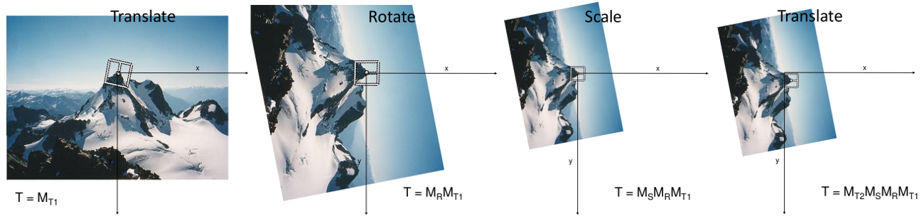
You will use cv2.warpAffine to perform the transformation. warpAffine takes a 2x3 forward warping afffine matrix, which is multiplied from the left so that transformed coordinates are column vectors. The easiest way to generate the 2x3 matrix is by combining multiple transformations. A sequence of translation (T1), rotation (R), scaling (S) and translation (T2) will work. Left-multiplied transformations are combined right-to-left so the transformation matrix is the matrix product T2 S R T1. The figures below illustrate the sequence.
3. Feature matching
Now that you have detected and described your features, the next step is to write code to match them (i.e., given a feature in one image, find the best matching feature in another image).
The simplest approach is the following: compare two features and calculate a scalar distance between them. The best match is the feature with the smallest distance. You will implement two distance functions:
- Sum of squared differences (SSD): This is the the squared Euclidean distance between the two feature vectors.
- The ratio test: Find the closest and second closest features by SSD distance. The ratio test distance is their ratio (i.e., SSD distance of the closest feature match divided by SSD distance of the second closest feature match).
Testing and Visualization
Testing
You can test your TODO code by running "python tests.py". This will load a small image, run your code and compare against the correct outputs. This will let you test your code incrementally without needing all the TODO blocks to be complete.We have implemented tests for TODO's 1-6. You should design your own tests for TODO 7 and 8. Lastly, be aware that the supplied tests are very simple - they are meant as an aid to help you get started. Passing the supplied test cases does not mean the graded test cases will be passed.
Visualization
Now you are ready to go! Using the UI and skeleton code that we provide, you can load in a set of images, view the detected features, and visualize the feature matches that your algorithm computes. Watch this video to see the UI in action.
By running featuresUI.py, you will see a UI where you have the following choices:
- Keypoint Detection
You can load an image and compute the points of interest with their orientation. - Feature Matching
Here you can load two images and view the computed best matches using the specified algorithms. - Benchmark
After specifying the path for the directory containing the dataset, the program will run the specified algorithms on all images and compute ROC curves for each image.
The UI is a tool to help you visualize the keypoint detections and feature matching results. Keep in mind that your code will be evaluated numerically, not visually.
We are providing a set of benchmark images to be used to test the performance of your algorithm as a function of different types of controlled variation (i.e., rotation, scale, illumination, perspective, blurring). For each of these images, we know the correct transformation and can therefore measure the accuracy of each of your feature matches. This is done using a routine that we supply in the skeleton code.
You should also go out and take some photos of your own to see how well your approach works on more interesting data sets. For example, you could take images of a few different objects (e.g., books, offices, buildings, etc.) and see how well it works.
Downloads
Skeleton code: Available on GitHub
Extra images: Look inside the resources subdirectory.
cs5670_python_env: Tutorial on how to set up cs5670_python_env
Virtual machine: As an alternative to cs5670_python_env, the class virtual machine available here has the necessary packages installed to run the project code.
To Do
We have given you a number of classes and methods. You are responsible for reading the code documentation and understanding the role of each class and function. The code you need to write will be for your feature detection methods, your feature descriptor methods and your feature matching methods. All your required edits will be in features.py.
The feature computation and matching methods are called from the UI functions in featuresUI.py. Feel free to extend the functionality of the UI code but remember that only the code in features.py will be graded.
Details
-
The function detectKeypoints in HarrisKeypointDetector is one of the main ones you will complete, along with the helper functions computeHarrisValues (computes Harris scores and orientation for each pixel in the image) and computeLocalMaxima (computes a Boolean array which tells for each pixel if it is equal to the local maximum). These implement Harris corner detection. You may find the following functions helpful:
- scipy.ndimage.sobel: Filters the input image with Sobel filter.
- scipy.ndimage.gaussian_filter: Filters the input image with a Gaussian filter.
- scipy.ndimage.filters.maximum_filter: Filters the input image with a maximum filter.
- scipy.ndimage.filters.convolve: Filters the input image with the selected filter.
-
You will need to implement two feature
descriptors in SimpleFeatureDescriptor
and MOPSFeaturesDescriptor classes. The describeFeatures function
of these classes take the location
and orientation information already stored in a set of key points (e.g.,
Harris corners), and
compute descriptors for these key points, then store these
descriptors in a numpy array which has the same number of rows as
the computed key points and columns as the dimension of the feature (e.g., 25 for the 5x5 simple feature descriptor).
For the MOPS implementation, you should create a matrix which transforms the 40x40 patch centered at the key point to a canonical orientation and scales it down by 5, as described in the lecture slides. You may find the functions in transformations.py helpful, which implement 3D affine transformations (you will need to convert them to 2D manually). Reading the opencv documentation for cv2.warpAffine is recommended.
- Finally, you will implement a function for matching features. You will implement the matchFeatures function of SSDFeatureMatcher and RatioFeatureMatcher. These functions return a list of cv2.DMatch objects. You should set the queryIdx attribute to the index of the feature in the first image, the trainIdx attribute to the index of the feature in the second image and the distance attribute to the distance between the two features as defined by the particular distance metric (e.g., SSD or ratio). You may find scipy.spatial.distance.cdist and numpy.argmin helpful when implementing these functions.
-
Create a short report (details below), which includes benchmarking results in terms of ROC curves and AUC on the Yosemite dataset provided in the resources directory. You may obtain ROC curves by running featuresUI.py, switching to the "Benchmark" tab, pressing "Run Benchmark", selecting the directory "resources/yosemite" and waiting a short while. Then the AUC will be shown on the bottom of the screen and you may save the ROC curve by pressing "Screenshot". You will also need to include one harris image. This is saved as harris.png, every time the harris keypoints are computed.
Coding Rules
You may use NumPy, SciPy and OpenCV2 functions to implement mathematical, filtering and transformation operations. Do not use functions which implement keypoint detection or feature matching.
When using the Sobel operator or gaussian filter, you should use the 'reflect' mode, which gives a zero gradient at the edges.
Here is a list of potentially useful functions (you are not required to use them):
scipy.ndimage.sobelscipy.ndimage.gaussian_filterscipy.ndimage.filters.convolvescipy.ndimage.filters.maximum_filterscipy.spatial.distance.cdistcv2.warpAffinenp.max, np.min, np.std, np.mean, np.argmin, np.argpartitionnp.degrees, np.radians, np.arctan2transformations.get_rot_mx(in transformations.py)transformations.get_trans_mxtransformations.get_scale_mx
What to Turn In
Code:
Upload your features.py to CMS.
If you attempted extra credit action item 1 (see below), then upload your features_scale_invariant.py and readme_scale_invariant.txt to CMS. If you attempted the extra credit action item 2 (see below), then upload the extra credit version of features.py as extracredit.py and extracredit_readme.txt, describing your changes to the algorithm in detail. If you did not attempt the extra credit then you do not need to upload extracredit.py or extracredit_readme.txt (please do not upload empty files).
Report:
Create a report in form of a pdf document or a small website describing your work and submit it to CMS as report.zip. Within report.zip, there should be either an index.html file (along with any embedded files e.g. images) that we can open in a web browser or a report.pdf file containing the following deliverables:
- Run the benchmark in featuresUI.py on the Yosemite dataset for the four possible configurations involving Simple or MOPS descriptors with SSD or Ratio distance. Include the resulting ROC curves, report AUC and comment which method is the best.
- Include the harris image on yosemite/yosemite1.jpg. Comment on what type of image regions are highlighted. Are there any image regions that should have been highlighted but aren't?
- Take a pair of your own images and visually show feature matching performance of MOPS + Ratio distance, by including a screenshot from featuresUI.py feature matching tab.
- (If you did extra credit) Describe how you made your descriptor scale invariant and why it works.
- (If you did extra credit) Include the ROC curve and report AUC from Yosemite dataset with your custom algorithm using ratio distance. Describe your changes to the algorithm and why they improve performance.
Extra Credit
Action Item 1
Once you have completed all of the above tasks, fork your features.py and save it as features_scale_invariant.py. In this file, you will improve your implementation of describeFeatures in MOPSFeatureDescriptor by making the descriptor scale-invariant. This means that instead of scaling down the 40x40 window to 8x8 by a constant factor of 1/5, you will derive this factor adaptively. How you do it is your design choice, but it should be well motivated. You may refer to MOPS paper for one approach. You may choose to implement that, something else, or invent your own approach. Describe your implementation in readme_scale_invariant.txt, explaining how the descriptor works.
Action Item 2We will give extra credit for solutions (feature detection and descriptors) that improve mean AUC for the ratio test by at least 15%. A 15% improvement is interpreted as a 15% reduction in (1 - AUC). i.e. the area above the curve. Here is one suggestion (and you are encouraged to come up with your own ideas as well!)
 Implement adaptive
non-maximum suppression (MOPS paper)
Implement adaptive
non-maximum suppression (MOPS paper)
If you attempt the extra credit then you must submit two solutions to CMS. The first solution will be graded by the project rubric so it must implement the algorithm described in this document. Extra credit solutions should include a readme that describes your changes to the algorithm and the thresholds for each benchmark image. The submitted code will be checked against this description. Extra credit submissions which do not improve mean AUC by at least 15% will not be graded. You can measure your mean AUC by running the UI benchmark on the 5 datasets (bikes, graf, leuven, wall, yosemite). We will specifically check performance on the yosemite dataset.
The extra credit will be given based on the merit of your improvement and its justification. Simple hyperparameter changes will receive less extra credit than meaningful improvements to the algorithm.
It is important that you solve the main assignment first before attempting the extra credit. The main assignment will be worth much more points than the extra credit.
Acknowledgements
The instructor is extremely thankful t Prof. Steve Seitz for allowing us to use their project as a basis for our assignment.
Last modified on February 15, 2019