Assignment 1. Ray Tracing
Table of Contents
- 1 Requirements
- 2 Implementation guidelines
- 2.1 Hear me now and believe me later!
- 2.2 Compile your own executable.
- 2.3 Ray trace one triangle.
- 2.4 Ray trace a bunny.
- 2.5 Compute simple shading and import scenes with cameras and many meshes
- 2.6 Make the interactive version
- 2.7 Compute shading from point lights with Microfacet material
- 2.8 Compute shading from area lights with Microfacet material
- 2.9 Compute illumination from ambient light
This course is about interactive graphics, and much of it is about doing realistic rendering efficiently. In order to properly understand and use the various methods for efficient rendering, it’s important to know what the right answer is that is being computed; the purpose of this assignment is to build a simple reference that computes correct surface illumination from point, area, and ambient lights.
In this assignment we will use ray tracing, since it is the simplest way to compute accurate answers in the general case, and since this is an interactive graphics class we will make some effort to achieve reasonable performance by using a high-performance CPU-based ray tracing library. Note that current graphics hardware also supports hardware accelerated ray tracing at about 2 orders of magnitude higher performance, and these ray tracing methods are beginning to be used for the trickier shading computations in interactive systems (games) when they are running on the latest hardware. The role of ray tracing in interactive graphics is likely to increase, which is another reason to use ray tracing in this assignment.
Your mission is to build a simple ray tracer that can render a scene containing meshes illuminated by point lights, rectangular area lights, and ambient light. You will be building this program in C++ using a collection of libraries we provide; some are standard external libraries, some are built just for this course to make the specific goals of this assignment easier to achieve with less code. The external libraries include:
- Embree, Intel’s collection of high performance ray tracing kernels. It provides a quite simple interface that makes it easy to get started, and also provides the parallel and streaming kernels needed to get to higher performance.
- Assimp (stands for “asset importer”), a popular open-source library for reading scenes. It supports lots of scene formats and puts the mesh and hierarchy data into a simple lowest-common-denominator structure that it’s easy to read it from.
- Nanogui, a minimal user interface framework on top of OpenGL. It provides cross-platform UI with no need for any help from the native window system.
- STB, a header-only library providing very simple versions of common graphics needs such as image i/o.
- cpplocate, to simplify finding our assets.
- GLM, a vector math library that uses conventions identical to GLSL.
The libraries we are providing for this course include:
- GLWrap, which provides some simple wrappers around OpenGL objects to support writing OpenGL code in a reasonable C++ style.
- RTUtil, which provides a number of functions for input parsing, geometric computations, reflectance models, and random sampling, as well as ImgGUI, a simple app built on GLWrap and Nanogui that provides the ability to display an image in a window.
1 Requirements
To successfully complete this assignment you have to build a ray tracer in C++, using Embree for ray tracing, with the following features:
- The executable takes a single command line argument that is the filename of a scene in OBJ, Collada, or GLTF format.
- If there are any cameras in the scene, the first camera will be used. Otherwise the default camera is at (3,4,5) looking at (0,0,0) with y up and a 30 degree horizontal FOV.
- The scene consists of all triangle meshes in the input scene. Other geometry can be ignored.
- The illumination comes from lights found in the scene, which can be point and directional lights, rectangular area lights (one-sided Lambertian emitters), or constant environment lights (ambient lights).
- Materials are specified in the input and are interpreted as physics-based materials using a microfacet model with a Beckmann normal vector distribution.
When the executable runs, it brings up a window and traces rays in batches of one ray per pixel, updating the image after each batch. Some kind of mouse-based camera control is available to change the view, with the image resetting each time the camera is moved. After N batches with the camera stationary, the window should correctly display the result of N rays per pixel. At every multiple of 64 rays per pixel, the program writes out a PNG image named in the format “render_sceneName_00256.png” (example for a render of the scene “sceneName.obj” with 256 samples per pixel) that contains the current image tonemapped linearly to 8 bits with sRGB quantization.
In addition, you should create:
- One cool “hero image”, which is a rendered scene of your choice with lighting set up however you like.
To demonstrate your successful implementation, you’ll do three things:
- Each week until the deadline, submit a 1-minute video demonstrating the current state of your assignment. These videos are graded on a yes/no basis based on whether they show substantial progress similar to the checkpoints noted in the assignment description below.
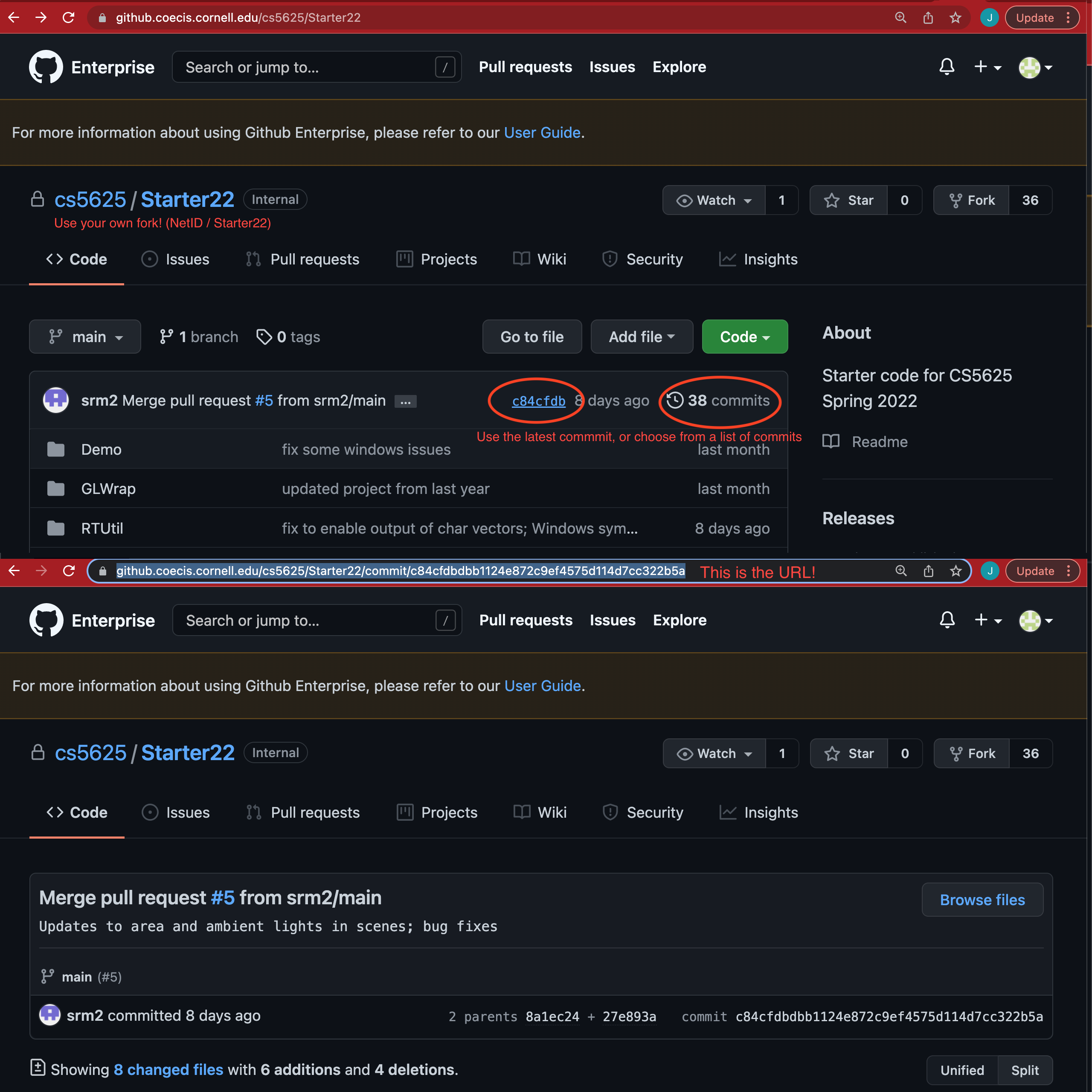
- Before the deadline, submit your C++ code by providing a link to the particular commit of your GitHub repo that you want to hand in. Here is an image demoing how to find this URL.
- Before the deadline, submit your output images for our test scenes with 256 samples per pixel, and your hero image.
- By one day after the deadline, submit a 2- to 5-page PDF report and
a 2- to-5-minute video demo that cover the following topics:
- The design and implementation of your program.
- What works and doesn’t, if not everything works perfectly. This could include illustrations showing that you successfully achieved some of the intermediate steps in our guidelines.
- How you made your hero image.
Grading will be based primarily on 3 and 4 – we don’t guarantee we will figure out how to compile and run your program, so it’s your job to submit the evidence on which I’ll base your grade.
2 Implementation guidelines
You have complete freedom to implement the assignment however you want; the only requirement is to code in C++ and to use Embree. If you are excited about some particular approach, or just want to take control of the design of your program, feel free to disregard our recommendations below (probably after reading them anyway since they contain a lot of useful hints!). But if you are newish to C++, a little uncertain about the material, are short on time, want to minimize risk, or tried plan A and ran into problems you weren’t able to solve, these tutorial-style guidelines are designed to help you get from zero to working implementation with as little frustration as possible.
2.1 Hear me now and believe me later!
Completing this assignment requires using building a fair bit of code (our solution is around 800 LOC), with no working framework to start from. C++ is also a rather error-prone language, with fewer safeguards than, say, Java or Python, and it’s just the nature of the language that it is easy to create hard-to-find bugs. Therefore it’s crucial to implement stepwise and test as you go—you should never do more than 15 minutes of coding before reaching a state where you can compile and test your program. Really! If you spend 2 hours implementing, and then try to debug what you have created, you are in for wasting a lot of time. You want steady progress, and progress is measured in terms of working code, not in terms of “finished” code that has not been tested (and therefore can be presumed to be full of errors).
2.2 Compile your own executable.
Create a subdirectory called RTRef (or whatever you want
to call it), and add an executable referring to that directory at the
end of CMakeLists.txt. Create a C++ source file with a
hello-world main() function. Running make again (from the
build/ directory) should now compile your program and you should be able
to run it as ./RTRef.
2.3 Ray trace one triangle.
In this step, we use Embree to build a (very) simple ray tracer. Take a look at the documentation for the Embree API, paying particular attention to the basic functions relating to Device, Scene, and Geometry objects. In particular, you’ll need:
rtc{New,Release}Device,rtc{New,Release}Scene,rtc{New,Release}Geometryto create and free things;rtcAttachGeometryto place geometry into the scene andrtcCommit{Geometry,Scene}to let Embree know we have added stuff;rtcSetNewGeometryBufferto set up triangle mesh data;rtcInitIntersectionContextandrtcIntersect1to trace rays; andrtcSetDeviceErrorFunctionis very useful for learning about errors when they happen to avoid getting confused.
Setting up a triangle mesh involves associating a vertex position
buffer and a triangle index buffer with the Geometry, and there are a
few ways to achieve this but the simplest, illustrated by the example
referenced below, is to use rtcSetNewGeometryBuffer, which
allocates the buffer, associates it with the geometry, and gives you the
pointer so you can write the data into it. You can ignore the many other
functions about geometry and all the geometry types other than
RTC_GEOMETRY_TYPE_TRIANGLE.
- Take a look at the “minimal” demo
from the Embree tutorial
(you can also find this under
ext/embreein your own source tree), and replicate what they are doing there by copying the code to build the scene and trace two rays against it into a couple of functions called by yourmain(). Put a comment at the top of your file acknowledging this source, to be removed if/when there are no traces remaining of the tutorial code. - Their scene has a bounding box from (0,0,0) to (1,1,0) and they
trace rays parallel to
the axis. Write a ray tracing loop that makes a fixed-size image by tracing a grid of similar rays in the
direction originating on the square (-0.5, -0.5, 1) – (1.5, 1.5, 1) these will hit the triangle near the middle of the grid and miss it on all sides. Set the corresponding pixels to white or black depending on whether they rays hit.
To get the image out the door with a minimum of fuss, you can use the
stb_image_write library. Put your image in an array of type
unsigned char[NX*NY*3], then when the data is in it make a
single call to stbi_write_png
with a hardcoded filename. (The principal documentation for this library
is in the header comment. Note that stride_in_bytes means
the size of one row of the image in bytes.) You should get an image with
a triangle in it! reference
2.4 Ray trace a bunny.
Next let’s get the ray tracer working for more interesting scenes by using the Assimp library to read in some triangle meshes. The documentation for that libary is lower quality than Embree’s so I’ll explain a little more here. The documentation is available but you can also read the header files directly.
Assimp provides a pretty simple C++ interface consisting of a class
Assimp::Importer,
which has a method ReadFile that opens a file, decides what
format it is, reads it into an in-memory data structure, and optionally
applies post-processing steps like triangulating polygons, applying some
mesh fixes, etc. There are a bunch of other features here but really you
only need the one function. Note that the importer retains ownership of
the scene by default, so the Importer object needs to live
as long as you need to be able to access the scene. (This is a common
source of bugs in this assignment: you create the aiScene
as a local variable of a “LoadScene” function, then store pointers to
parts of its data structure in your own data structure, then return your
data structure. The aiScene and all its contents are
deallocated when the function returns, and at unknown times in the
future this data will be overwritten with random other stuff and cause
you to be very confused.)
The scene is an object of type aiScene,
which holds lists of the resources (meshes, materials, textures,
cameras, lights, etc.) in the scene and a node hierarchy that encodes
the transformations for all these objects. For our immediate purpose we
only want to get hold of the meshes in an OBJ file, so we can ignore the
node hierarchy (OBJ does not even support transformations, after all)
and just read the meshes directly.
- Following the example
in the documentation, create an
Importerand ask it to read from the OBJ file of the bunny inresources/meshes/bunny.obj. UsingaiScene::{HasMeshes, mMeshes, mNumMeshes}, iterate through the meshes and print out the number of vertices and triangles in each, along with a few vertex positions and face indices. Compile and test to be sure this is working and that the numbers look sane. - Now merge your single-triangle scene setup with this scene
traversal: create an
RTCScene, read in anaiScene, and then for each mesh in theaiScenecreate the correspondingRTCGeometry, copy the data from theaiMesh, commit it, and attach it to the scene. Use exactly the same sequence of calls as for the single triangle but don’t forget you will need to specify the size of the buffers tortcSetNewGeometryBuffer.
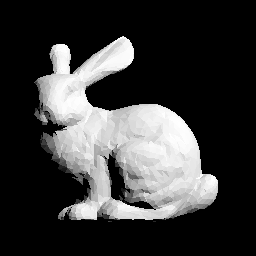
The bunny is also roughly the size of the unit cube, so you should see the silhouette of a bunny in your output! reference (original view) reference (more sensible view)
This is the checkpoint for Week 1. You should have this much working on Feb 17 and hand in a very short video showing it off.
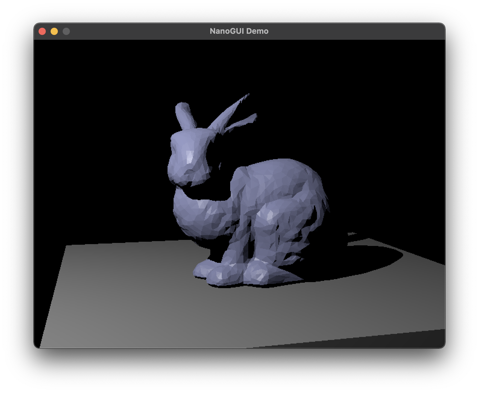
2.5 Compute simple shading and import scenes with cameras and many meshes
This step will use the last of the major tools for this assignment,
the GLM vector library. Familiarize yourself with the use of
glm::vec3, glm::mat4, and friends: how to
initialize them, how to compute scalar and dot products and
matrix-matrix and matrix-vector products. The design goal of GLM is for
its usage to be sufficiently analogous to the GLSL vector and matrix
types that you are already familiar with it. Note that we provide output
operators for GLM vector and matrix types in
RTUtil/output.hpp, which is convenient for debugging
output.
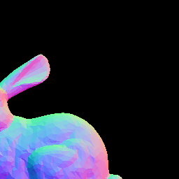
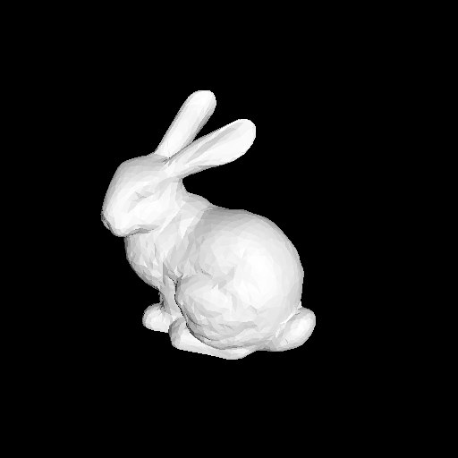
First you need normals, which Embree provides in the RayHit structure. Render a normal-shaded bunny to check them. reference
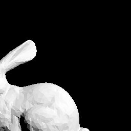
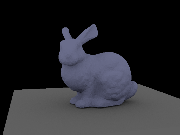
Implement simple diffuse shading with a fixed directional light source in the direction (1,1,1), and verify you can get a nice looking (though faceted) shaded bunny. reference (original view) reference (sensible view)
The lack of a controllable camera is starting to be an annoying limitation, so let’s fix things to use the camera that is in the input scene (if there is one). The Assimp scene contains a list of cameras; just use the first one if there is one, otherwise the default camera from the requirements above. You’ll probably want to create a simple camera class that supports ray generation for a basic perspective camera. (See CS4620 for a refresher.)
First make sure this works with the bunny OBJ file and the default
camera. reference Then, to
get a scene with a camera in it, try scenes/bunnyscene.glb;
it is a GLTF file exported from Blender, which has the bunny mesh in it
along with a floor, a camera, and a couple of lights. (The scene is in
scenes/bunnyscene.blend and Blender is here if you want to change
it).
Before this is going to work right, though, you need to account for
the transformations that are applied to objects in the scene, including
the camera. The aiScene that the importer provides you has
a node
hierarchy as well as the lists of meshes, cameras, etc. Each object
that is actually in the scene is referenced from a node in the
hierarchy.
For the camera, since we are selecting the camera as the first one in
the list,
the way to find its transformation is to find the node for the camera by
name (using aiNode::FindNode),
then walk up the node hierarchy by following the parent pointers up to
the root. (The approach is summarized
in the header comment for the aiCamera class, though I find
it more natural to accumulate the transformations starting from the node
and going up toward the root).
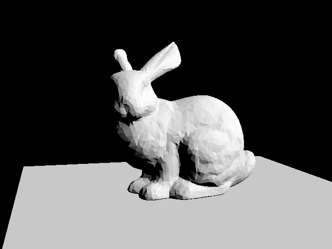
For the meshes, since meshes might be used zero times or more than once, you should not start from the list of meshes, but instead traverse the node hierarchy, and for each node that has meshes in it, transform the vertices of the mesh by the node-to-world transformation.
Once this all works you should be able to render a view of the bunny sitting on the floor. reference (before adjusting pixel count to match camera aspect) reference (after)
A couple hints about GLM:
- Generally, you can assume the interface to be pretty similar to that
of GLSL. One exception to that is vector swizzling. For example, in
GLSL, if you want to truncate a
vec4to avec3, the simplest way to do that would bemyvec4.xyz, however, in GLM, prefervec3(myvec4). - Don’t forget to
#include <glm/glm.hpp>, as well as to use theglm::namespace! - GLM also provides helpful matrix utilities in
<glm/gtc/matrix_transform.hpp>. - The definitive resource is always the documentation.
Assimp has its own matrix/vector types, which are fine, but we
preferred to be consistent about using GLM in our implementation. So we
wrote simple conversion functions that we are providing in
RTUtil/conversions.h: you can write
glm::thing = a2g(aiThing) for a variety of things including matrices and vectors of all the necessary types and sizes.
2.6 Make the interactive version
Since our whole point in this course is interactive graphics, we should make this renderer interactive. With simple shading it should be running pretty fast, so let’s make it display in real time.
Since what you’ve written so far operates in batch mode, this may be a good opportunity to rearrange the code a little bit; perhaps move the ray tracing code into a separate source code file from the main function, if you haven’t already, and think a bit about how to provide yourself an interface that lets you load a scene and then render images of that scene. You’ll need to be able to call this from inside an interactive drawing loop, but you might like to keep the batch mode interface around at least for now. Don’t forget to compile and test frequently as you reorganize to ensure everything still works.
To create an interactive app that displays an image, you can use the
provided class ImgGUI:
- Define a subclass of
ImgGUI. - Override the member function
compute_imagewith something that fills the image with a fixed color. - In your main function, create an instance of this class and call
nanogui::mainloop; see theDemoapp for an example.
Get this much working; you should get a constant colored window. Then:
- Provide a way to get the scene data that you loaded in the earlier
steps into your
ImgGUIsubclass. - Modify the function
compute_imageto do basically the same thing as your batch renderer, writing the result into the arrayimg_data.
Once this works you should see the same image you computed before, displayed in the window.
At this point it is irresistable to implement camera control so you
can spin your bunny around. You can get hold of the necessary events by
overriding the methods nanogui::Widget::mouse_button_event,
nanogui::Widget::mouse_motion_event, and
RTUtil::ImgGUI::keyboard_event. There are no detailed
specifications for this part; you should implement camera control that
you find useful. Two approaches that can work well:
- Apply transformations to the camera for each mouse motion or keyboard event that you wish to respond to. For instance, rotate the camera around its local origin and translate it along its view direction, to implement “fly” semantics. You might need to do something to keep the camera upright.
- Keep track of spherical coordinates for the camera position relative to a target point (maybe the origin, though it’s nice if it’s a point that the initial camera is looking at). Update the spherical coordinates at each event, then recompute the camera’s position and direction. This is a pretty effective way to implement “orbit” sematics.
2.7 Compute shading from point lights with Microfacet material
Now we are at a position to get to the algorithmic meat of the assignment (not that learning how all these APIs work isn’t also part of the goal).
The first thing you will need is the lights. Just like meshes, you
will need to use the aiScene::{HasLights, mLights,
mNumLights} fields. Note that lights also have transformations,
and lights and transformations are associated in the same way as cameras
and transformations.
Unfortunately, our primary file format (GLTF) does not support area and ambient lights, which we would like to have. Thus we will sneak the extra information in via the names of the lights using this logic:
- If the light’s name starts with
Ambient_r<distance>, it is an ambient light with the fieldmColorAmbientas its radiance and<distance>as its range. - If the light’s name starts with
<name>_w<width>_h<height>, then it is a constant-radiance one-sided area light called<name>with size<width>(x) by<height>(y) (both of which should be interpreted as floats) in its local coordinates. The center is atmPositionand it is facing in the+zdirection (which of course might end up being a different direction once you do the appropriate transformations). The total power of the light ismColorDiffuse(ignore the misleading name - assimp uses an old school light model). - Otherwise, it is a point light with power
mColorDiffuse.
When analyzing the names you should ignore any trailing characters,
since exporters love to append extra stuff to the names of objects. We
have provided two functions in RTUtil/conversions.hpp to
help with this. The functions parseAreaLight takes a string
as input and returns a boolean that is true if the string matches the
area light format above, and in this case it fills in the
width and height output arguments. The Ambient
light works similarly.
The other thing you need for surface shading is materials. We suggest starting by just using a default material for all surfaces, and returning to this after shading is working.
For this part only compute illumination from point lights. This is a simple computation that does not require any integration: compute the direction and distance to the light, evaluate the surface’s BRDF for the view and light directions, and compute
where is the intensity of the light source,
computed from its given power, and
and
are the view
and light directions. Of course you will want to wrap this in a standard
shadow ray test. (For this test note that you can save a little bit of
time by using
rtcOccluded1 instead of
rtcIntersect1 to test for the intersection.)
To evaluate the BRDF we have provided a small class hierarchy as part
of RTUtil that is borrowed from Nori,
an educational raytracer. It includes a base class BSDF and a single
implementation Microfacet, which is a material with Lambertian diffuse
and microfacet specular reflection. The method BSDF::eval
can be used to compute BSDF values for given illumination and viewing
directions (you have to set up a BSDFQueryRecord and pass
it in). A key thing to realize, though, is that this class expects these
directions to be in the coordinates of a surface frame with the
first two coordinate directions tangent to the surface and the third
direction normal to the surface. At first you will have these vectors in
world coordinates, and you need to build a basis for the surface frame
and transform these vectors into this basis. The class
nori::Frame is useful for this computation; it can build a
basis from just the surface normal and transform directions between this
frame and world coordinates.
Once this shading works with a single default material (reference with diffuse color
(0.2, 0.5, 0.8), roughness 0.2, index of refraction 1.5), then get the
selection of different materials working. To do this, you need to make
use of Embree’s features for associating data with Geometry objects in a
scene. There are two mechanisms: geometry can be assigned integer IDs
when added to the scene (rtcAttachGeometryByID), or a
user-defined pointer can be associated with gometry
(rtcSetGeometryUserData). Either will work fine; I used the
integer IDs and a std::map that maps these IDs to
materials.
Assimp divides meshes up so that each mesh has a single material. The
materials are all stored in the aiScene::mMaterials array,
and you can associate a mesh with a material by indexing into that array
with the index provided in the aiMesh::mMaterialIndex
field. To access specific properties of the material, you can do
mat->Get(<material-key>, <where-to-store>).
The specific material properties we care about for our microfacet model
are AI_MATKEY_ROUGHNESS_FACTOR and
AI_MATKEY_BASE_COLOR.
For example, you might do this to get the base color:
glm::vec3 color;
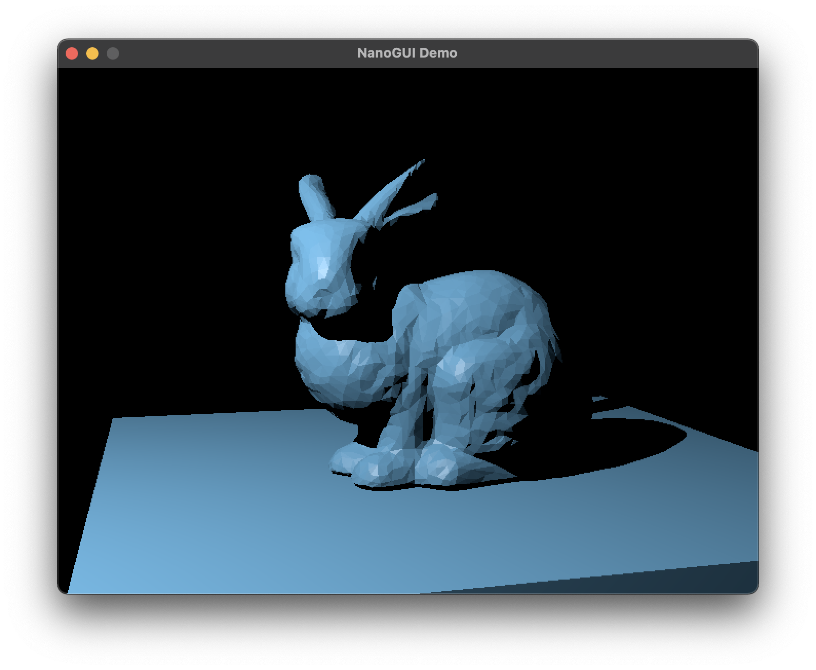
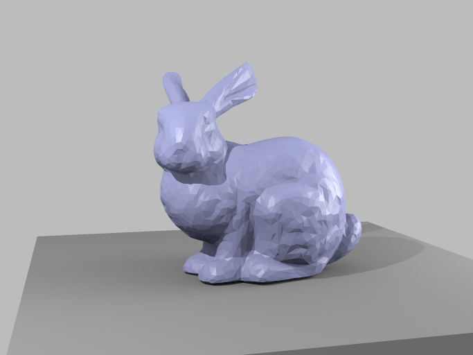
mat->Get(AI_MATKEY_BASE_COLOR, reinterpret_cast<aiColor3D&>(color)); # cast our vec3 to what assimp expects - its color typeOnce this works, from bunnyscene.glb you should be able
to render a rather harshly lit blue bunny on a gray table with a shadow
and microfacet highlights, and there’s no reason it shouldn’t render at
interactive rates as you move the camera. Here is a reference for this.
This is the checkpoint for Week 2. You should have this much working on Feb 24 and hand in a very short video showing it off.
2.8 Compute shading from area lights with Microfacet material
The next type of light to get working is area lights. The code for this is quite similar to that for point lights but is a bit more subtle. In this case (see the lecture slides) we are estimating the value of a definite integral
where is the
shading point,
is a point on
the light source, and
is the direction from to
. Estimate
this integral by choosing
from a
uniform random distribution over the surface of the source; this means
where
is the area of the source. See the
slides for more detail on defining an estimator for this integrand and
this
. Here is a one-sample reference.
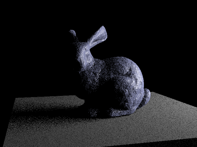
Finally, change your program so that it continuously computes images
and accumulates them, as described in the requirements. This means that,
as long as the camera is not moving, the newly computed pixel values are
averaged into the existing image in such a way that after waiting for
frames, the user is looking at an image
rendered with
samples per light. You will want to
reset the sample count when the camera moves so that the old image data
is forgotten. Also set it up to write out images periodically as
described in the requirements above. Here is a reference image with 256 samples.
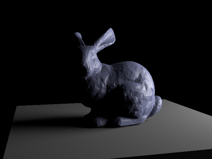
2.9 Compute illumination from ambient light
The last component of lighting for this assignment is an ambient component to fill in shadows. This is like lighting from an environment light, but to keep things simple we have two simplifications: the ambient light is constant in all directions, and it only illuminates the diffuse component of the BSDF. This serves to provide pleasant soft illumination that simulates indirect light, but without making it difficult to keep the variance low.
The other feature of our ambient light is ambient
obscurance. The idea is that nearby surfaces prevent ambient light
from reaching our shading point, but if they are too far away we ignore
them (otherwise interior scenes would have no ambient light). The
ambient lighting model has two parameters: the radiance of the ambient light and the
range
beyond which occlusion is not
counted.
To estimate ambient illumination we use the integral for illumination of a diffuse surface by an environment:
Here is the BRDF value for just the
diffuse component, which can be computed from the diffuse reflectance
that is available from
BSDF::diffuseReflectance, and is
the occluded ambient light:
This integral can be estimated by Monte Carlo, using cosine
distributed samples. You will find the function
RTUtil::squareToCosineHemisphere useful for generating
these samples (but don’t forget to transform them to global
coordinates).
If you enable only the ambient light, you will get very soft illumination that resembles an overcast day. The Bunny scene has unlimited obscurance range, which leads to ambient occlusion; here are references with 1 and 256 samples.
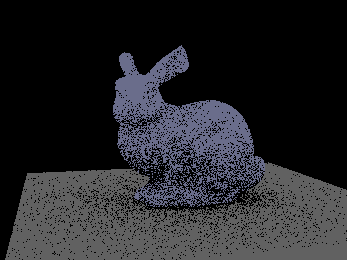
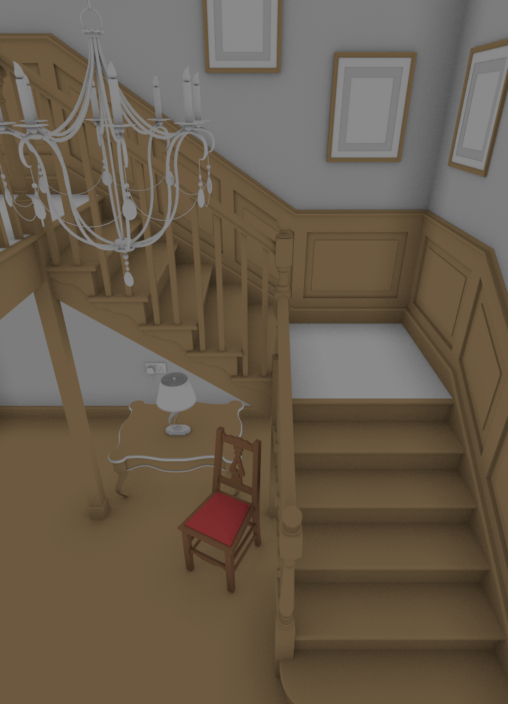
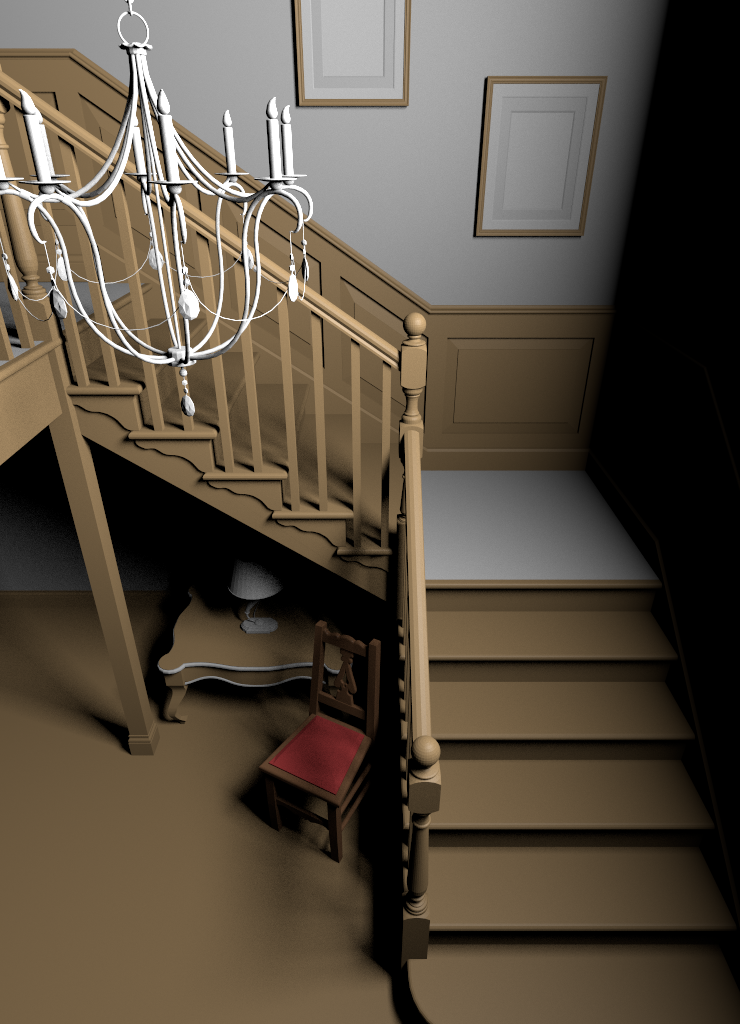
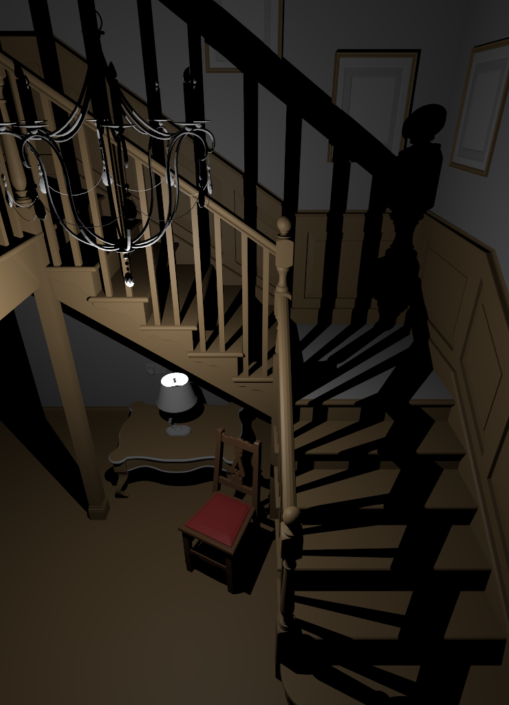
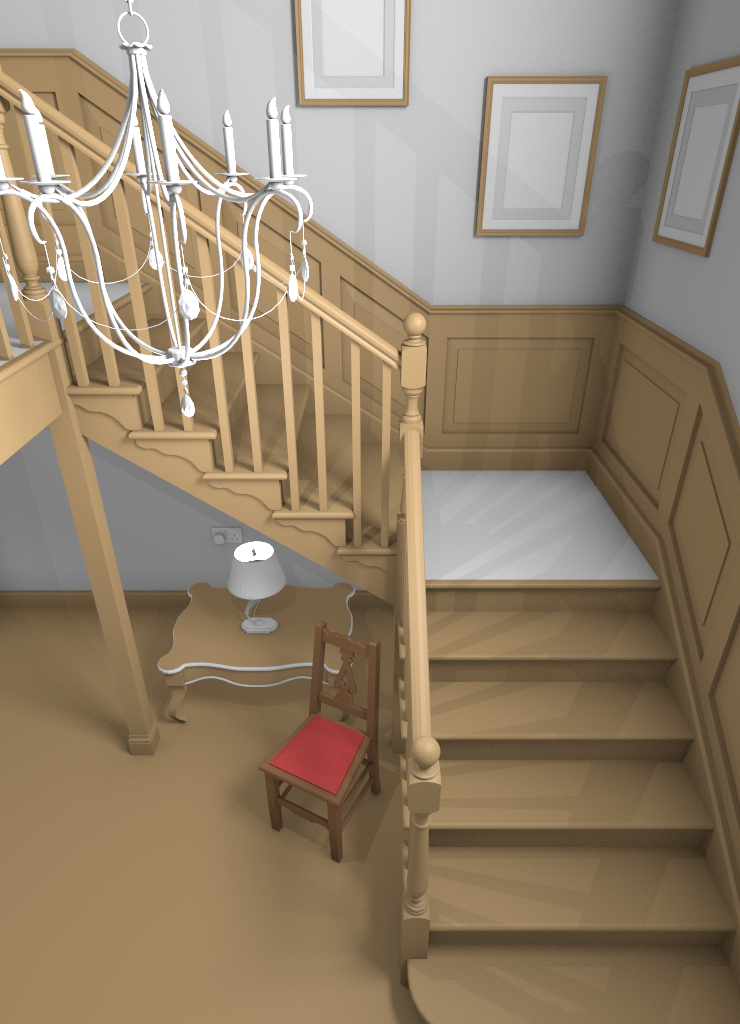
Now that everything works, you can enable all the lights and explore
what your renderer can do! Here are references for the bunny with the given camera, and
for the scene staircase.glb from the default view with ambient
only, area
only, point
only, and with all three
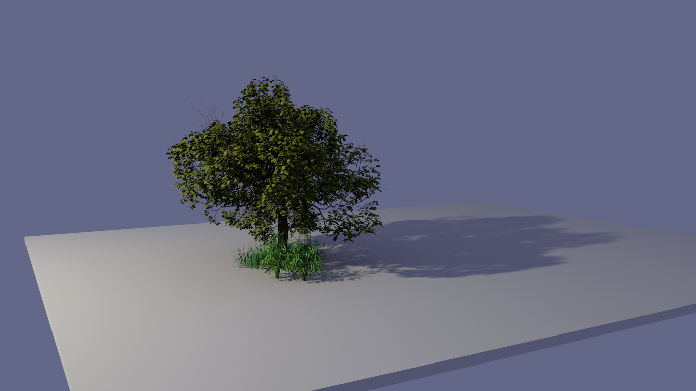
lights. Finally, there is a scene tree.glb that has
more polygons in it; here is a reference. For the
tree scene you will find the leaves are single-sided, so to get a nice
rendering your shading code will need to be willing to shade both backs
and fronts of surfaces; this is easy to arrange by simply negating the
normal if you find it is facing away from the view direction. (This also
makes it easier to render random scenes from the web since people are
not always careful to keep their surfaces oriented consistently, and
it’s harmless until you want to do materials like glass).
And finally, don’t forget about making a nifty hero image. Your scene doesn’t have to be terribly complex, but explore the internet for models or scenes (Blend Swap, TurboSquid, McGuire, Crane, Stanford, …) and play with the scene setup and lighting to make something you like! Blender is a good tool for this, and if you export to GLTF format, ensure all geometry is meshes, be sure to ask it to export cameras and lights, and ensure the first camera in the scene is reasonable, you should have good luck reading them with your program.
Once you’ve reached the end, see the discussion at the beginning for what to hand in for this assignment.