CS5625 PA8 Soft Shadows

Out: Friday April 8, 2016

Due: Friday April 15, 2016 at 11:59pm

Work in groups of 2.

Overview

In this assignment, you will implement two techniques for soft shadows in interactive graphics application:

soft shadows from area lights using percentage closer soft shadows (PCSS), and
screen-space ambient occlusion (SSAO).

Task 1: Percentage Closer Soft Shadows

Edit

the appropriate branch of the getShadowFactor function in student/src/shaders/deferred/pa8_ubershader.frag

to implement Randima Fernando's percentage-closer soft shadows (PCSS) technique as it is described in this SIGGRAPH sketch. For more discussion of this method and how it relates to other methods, see these Eurographics course notes.

Your implementation should make use of the following uniforms in the shader:

spotLight_lightWidth: the 1D width of the light source in scene unit. The light source is a square whose size is of length spotLight_lightWidth centered at the point $(0,0,0)$ and lying in the $xy$-plane in the eye-space of the light source's camera.
spotLight_pcssBlockerKernelSampleCount: the number of samples to use when computing the average blocker depth. The default value is 40.

As you probably have read in the document, the first step of PCSS involves estimating the area in which you will sample the shadow map for depths of blockers. To do this, compute the length of the side of the light source if it were to be projected onto the near plane of the light source's camera. You will find that the spotLight_near and spotLight_fov are useful for this calculation. Let us denote the computed size by $s$, and let the unit of $s$ be shadow map pixels.

Next, you should sample spotLight_pcssBlockerSampleCount points from the shadow map in the square of side length $s$ around the point on the shadow map which corresponds to the position argument of the getShadowFactor function. Use the uniformly distributed random numbers in the unifRandTex texture to generate these points. You should then find the average of the $z$-coordinate of the samples that pass the shadow map test. Recall that Task 2 of PA7 directs you to store the (negative of the) $z$-coordinate of the geometry in the $w$-component of the shadow map texel. This is the value that should be used to compute the average blocker depth.

After getting the average $z$-coordinate of the blocker, you should use it to find the penumbra size as specified in the Fernando's paper. Use this penumbra size as the window size, evaluate PCF shadow factor like what you did in the last assignment, and return the result as the shadow factor for PCSS.

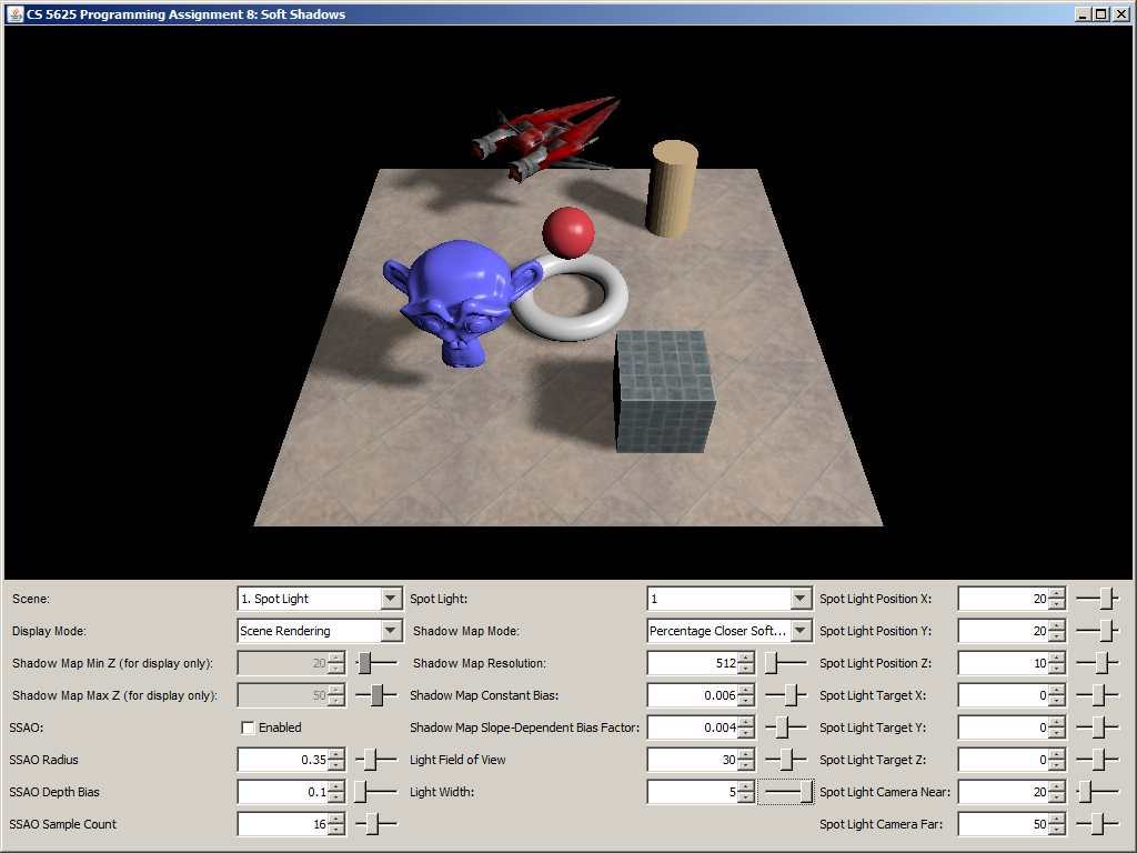
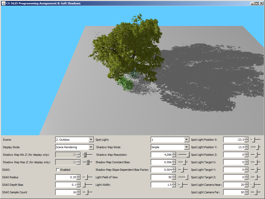
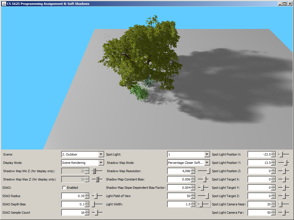
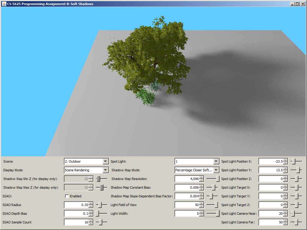
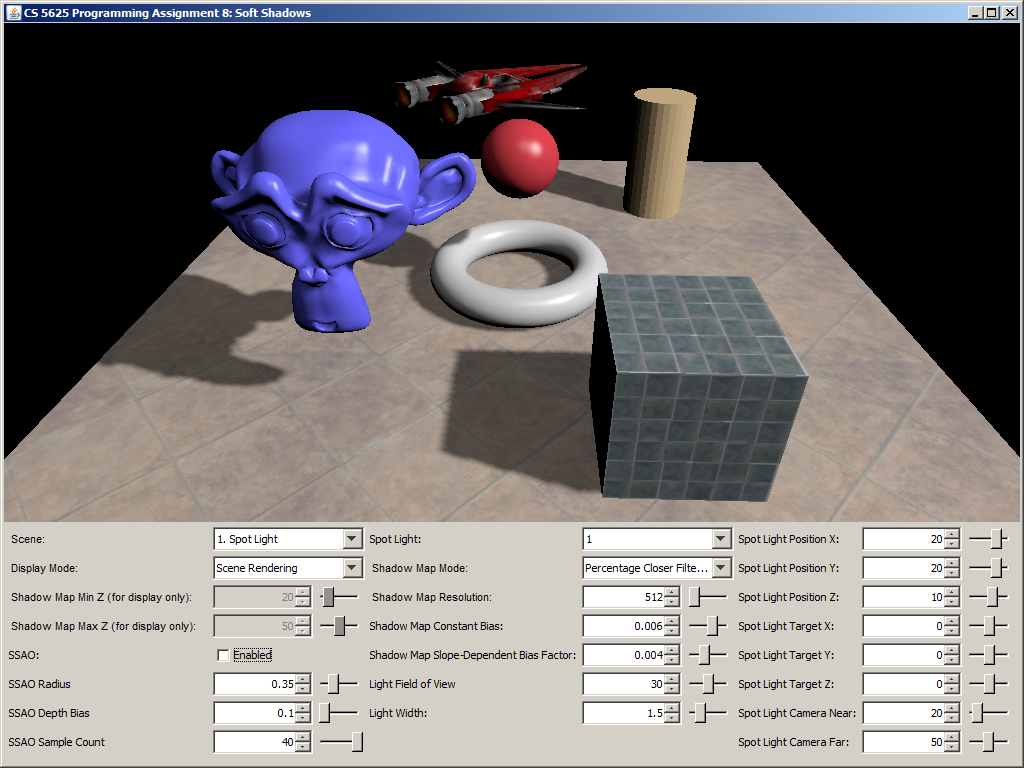
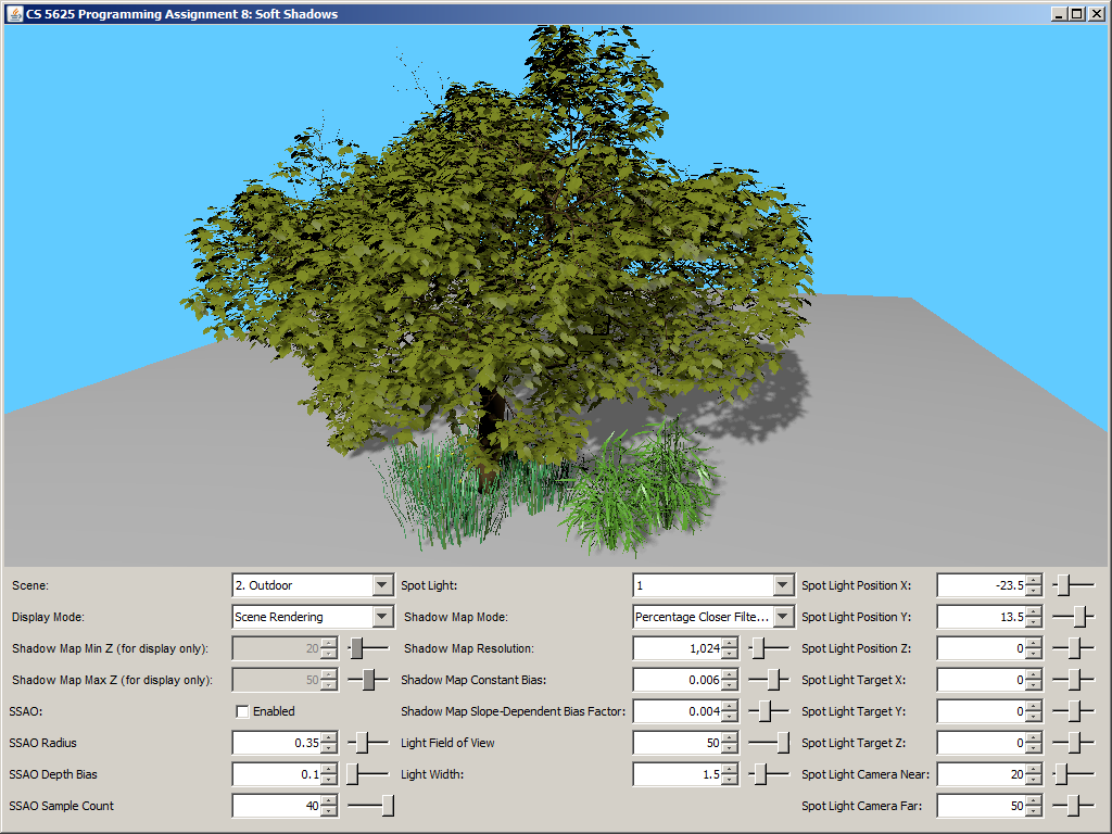
A correct implementation should yield a picture that looks like simple shadow mapping when the light width is set to 0. The shadow should then become more blurry as you increase the light size. Shadows that are further away from the shadow caster should be blurrier and larger.

Light width = 0	Light width = 1.5	Light width = 5

Task 2: Screen-Space Ambient Occlusion

Edit:

student/src/shaders/deferred/ssao.frag

to implement the screen-space ambient occlusion technique.

The shader above takes the 4 G-Buffers, their dimensions, and the following parameters as input:

ssao_radius: the radius of the hemisphere inside which to generate samples for SSAO.
ssao_depthBias: the bias for the depth read from the G-Buffers.
ssao_sampleCount: the number of SSAO samples to generate.
sys_projectionMatrix: the projection matrix that was used to render the G-Buffers.

It should output a grayscale pixel (i.e., all channel, except the A-channel, should have the same values) whose value approximates the integral: $$ \frac{1}{\pi} \int_H V(\mathbf{p}, \omega)\ (\mathbf{n} \cdot \omega)\ \mathbf{d} \omega $$ where

$\mathbf{p}$ is the eye-space position of the fragment being shaded,
$\mathbf{n}$ is the eye-space normal of the surface at $\mathbf{p}$,
$H$ is the unit hemisphere of direction centered at $\mathbf{p}$ and oriented along $\mathbf{n}$,
$\omega$ represents a direction, and
$V(\mathbf{p}, \omega)$ is the visibility function, which is $1$ if the ray from $\mathbf{p}$ in direction $\omega$ does not intersect any geometry in the scene and $0$ otherwise.

The value of the integral is called the ambient occlusion at point $\mathbf{p}$.

In this assignment, however, we will approximate the ambient occlusion with the ambient obscurance: $$ \frac{1}{\pi} \int_H V_r(\mathbf{p}, \omega)\ (\mathbf{n} \cdot \omega)\ \mathbf{d} \omega $$ where $V_r(\mathbf{p}, \omega)$ is 1 if there is no geometry intersecting the segment from $\mathbf{p}$ in direction $\omega$ of length $r = \mathtt{ssao\_radius}$, and 0 otherwise.

We shall approximate the above integral with Monte Carlo integration. We pick a probability distribution $p(\omega)$ on the hemisphere $H$ and generate $N = \mathtt{ssao\_sampleCount}$ samples of directions $\omega_1$, $\omega_2$, $\omega_3$, $\dotsc$, $\omega_N$ according to the distribution $p$. Then, the obscurance is approximated as follows: $$ \frac{1}{\pi} \int_H V_r(\mathbf{p}, \omega)\ (\mathbf{n} \cdot \omega)\ \mathbf{d} \omega \approx \frac{1}{\pi N} \sum_{i=1}^N \frac{V_r(\mathbf{p}, \omega_i)(\mathbf{n} \cdot \omega_i)}{p(\omega_i)}.$$ The calculation is the easiest to carry out if we pick $p$ so that $p(\omega)$ is proportional to $\mathbf{n} \cdot \omega$, causing the $(\mathbf{n} \cdot \omega_i)$ term of cancel out. By doing so, it also turns out that $p(\omega) = (\mathbf{n} \cdot \omega) / \pi$, so the calculation simplifies to: $$ \frac{1}{\pi} \int_H V_r(\mathbf{p}, \omega)\ (\mathbf{n} \cdot \omega)\ \mathbf{d} \omega \approx \frac{1}{\pi N} \sum_{i=1}^N \frac{V_r(\mathbf{p}, \omega_i)(\mathbf{n} \cdot \omega_i)}{(\mathbf{n} \cdot \omega_i) / \pi} = \frac{1}{N} \sum_{i=1}^N V_r(\mathbf{p}, \omega_i).$$ However, beware that the calculation works only when you generate samples according to the $p(\omega) = (\mathbf{n} \cdot \omega) / \pi$ distribution. See how to do so at the end of this writeup.

It remains to figure out how to compute or approximate $V_r(\mathbf{p},\omega_i)$. The idea is to sample a random point between $\mathbf{p}$ and $\mathbf{p} + r\ \omega_i$ (which is the intersection point between the ray from $\mathbf{p}$ in direction $\omega_i$ and the sphere of radius $r$ centered at $\mathbf{p}$) and see if the point does not lie beneath rendered scene geometry. More specifically, we compute the point $$ \mathbf{p}_i = \mathbf{p} + \xi\ r\ \omega_i $$ where $\xi$ is a random number in the range $[0,1]$ (which you can generate using the random function in the shader). You should then use sys_projectionMatrix to transform $\mathbf{p}_i$ to the corresponding texture coordinate of the G-Buffer and compute the corresponding eye-space position $\mathbf{p}'$ at that coordinate. We then compute $V_r(\mathbf{p}, \omega_i)$ by comparing the depth of $\mathbf{p}_i$ and $\mathbf{p}'$: $$V_r(\mathbf{p}, \omega_i) = \begin{cases} 1, & \mbox{if }|\mathbf{p}_i.z| \leq |\mathbf{p}'.z| + \mathtt{ssao\_depthBias} \\ 0, & \mbox{otherwise} \end{cases}.$$ In our implementation, we set $V_r(\mathbf{p}, \omega_i)$ to $1$ if $|\mathbf{p}_i.z| > |\mathbf{p}'.z| + \mathtt{ssao\_depthBias} + 5 \times \mathtt{ssao\_radius}$ so that the shaded point is not affected by objects that are too far away in front of it. In other words, we used the following equation: $$V_r(\mathbf{p}, \omega_i) = \begin{cases} 1, & \mbox{if }|\mathbf{p}_i.z| \leq |\mathbf{p}'.z| + \mathtt{ssao\_depthBias}\mbox{ or }|\mathbf{p}_i.z| > |\mathbf{p}'.z| + \mathtt{ssao\_depthBias} + 5 \times \mathtt{ssao\_radius}.\\ 0, & \mbox{otherwise} \end{cases}.$$

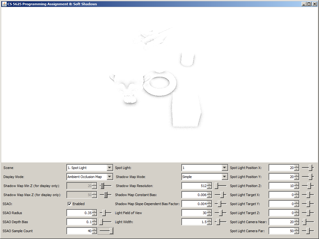
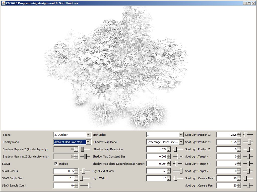
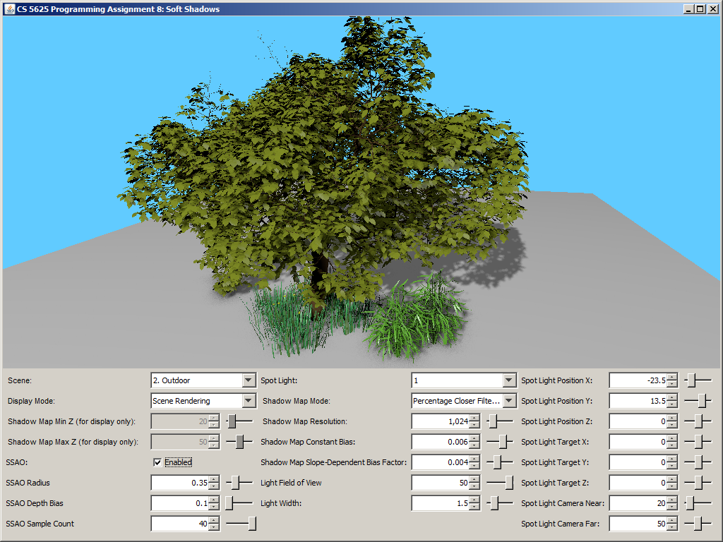
A correct implementation should yield the following results:

Ambient Occlusion Buffer	Rendering with SSAO	Rendering without SSAO

Sampling a point on the unit hemisphere according to $p(\omega) = (\mathbf{n} \cdot \omega) / \pi$

For simplicify, let us first assume that $\mathbf{n}$ is the positive $z$-axis. Our task becomes to generate a point $\omega = (x,y,z)$ where the probability of generating $\omega$ is $p(\omega) = (\mathbf{n} \cdot \omega) / \pi = ((0,0,1) \cdot (x,y,z)) / \pi = z/\pi.$ This can be accomplished by the following procedure:

Generate two random numbers $\xi_0$ and $\xi_1$ from the range $[0,1]$.
Compute: \begin{align*} x &= \sqrt{\xi_0} \cos(2\pi \xi_1) \\ y &= \sqrt{\xi_0} \sin(2\pi \xi_1) \\ z &= \sqrt{1-\xi_0} \end{align*}

You should get random numbers from the unifRandTex uniform.

Note that this gives you a point on the hemisphere that is oriented along the positive $z$-axis. However, what we really want to operate on is a hemisphere oriented along a general unit vector $\mathbf{n}$. An easy way to deal with this is to generate a point on the hemisphere oriented along $(0,0,1)$ first and then transform it to a coordinate system that has $\mathbf{n}$ as the positive $z$-axis. In our implementation, we also apply a random rotation around the $\mathbf{n}$ to the generated points to increase randomness.