CS5625 PA4 Mipmapping
Out: Friday March 4, 2015
Due: Friday March 11, 2015 at 11:59pm
Work in groups of 2.
Overview
In this programming assignment, you will implement:
- simple texture antialiasing operations,
- a mipmap pyramid with trilinear interpolation,
- high quality anisotropic texture filtering,
The notes on the framework listed at the beginning of PA3 apply to this assignment as well; in particular, the application renders continuously, attempting to take up all available CPU time. If you want a better behaved application when you are not worrying about framerate, you can modify the relevant GLView implementation for your platform, modifying it to use FPSAnimator at 30 or 60 frames per second rather than using the simple Animator class that redraws continuously.
Task 1: Texture antialiasing
The first task combines the two tasks in the last assignment to deal with the thorny problem of texture filtering. Classic references on this topic include the following papers:
L. Williams, “Pyramidal Parametrics,” SIGGRAPH 1983.
N. Greene & P. Heckbert, “Creating Raster Omnimax Images from Multiple Perspective Views Using the Elliptical Weighted Average Filter,” Computer Graphics & Applications 6:6 (1986).
The fragment shader that should contain the implementation for the sampling operations in this task is texfilter.frag. The test application is implemented by the PA4_Texfilter class that uses the associated renderer TexfilterRenderer.
Nearest-neighbor sampling
The first part of this task is fairly simple: when mode is MODE_BOX, perform nearest-neighbor sampling. Because the rectangle texture we are using doesn't support the GL_REPEAT wrapping mode, you'll have to wrap the coordinates yourself, as well as scaling them to texel coordinates. (Q: how does the performance differ if you do this using if statements vs. doing it using floating point functions?)
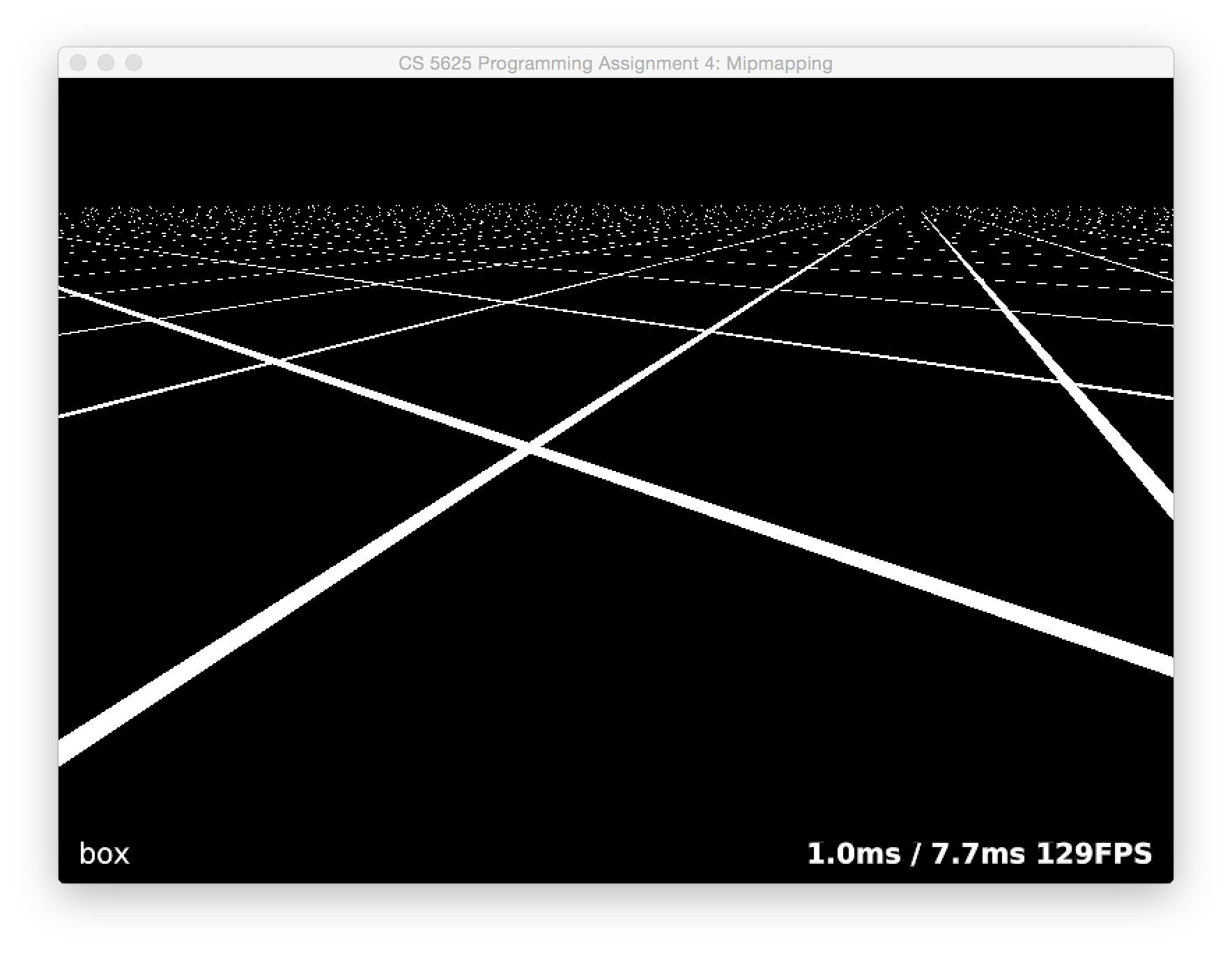
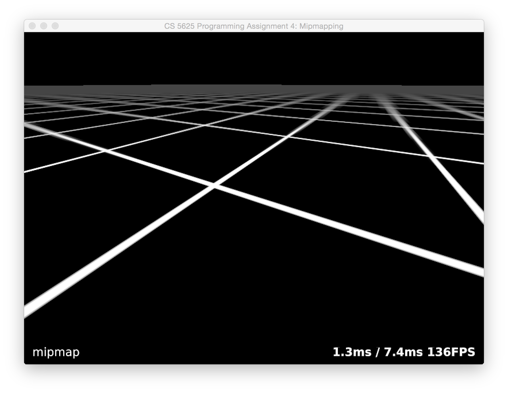
When you have this working, you should see a brick surface stretching to the horizon, and you should have a terrible mess of glittering, swimming Moiré patterns in the distance:

To see even more dramatic results, switch to the grid texture (use arrow keys to switch between textures):
Supersampling
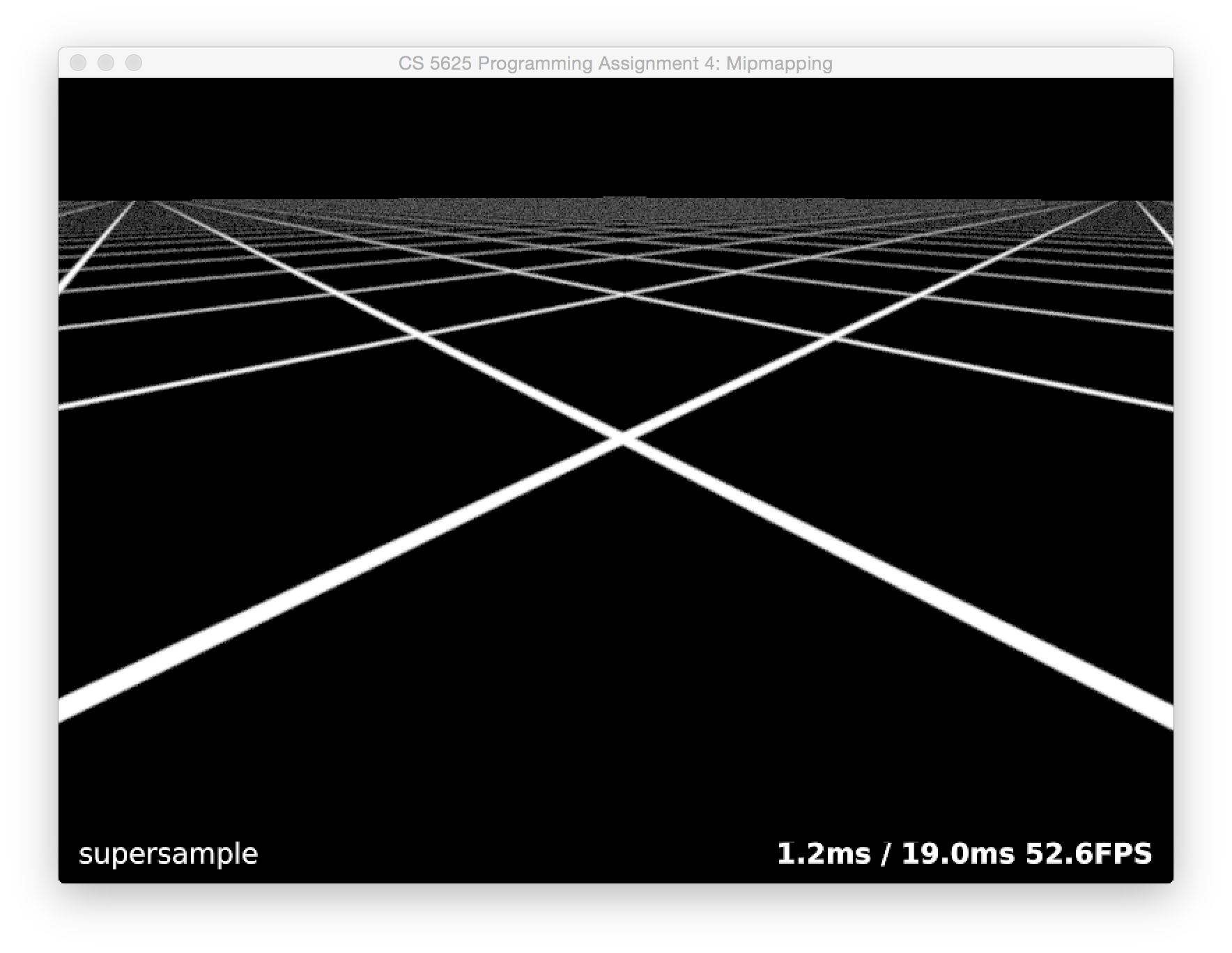
The simplest way to solve this problem is to average mutliple samples of the texture. You can do this in exactly the same way as you did supersampling for PA3. Use the Gaussian noise texture to take 80 samples per fragment and average them with Gaussian weights. Since we want the samples to cover an area corresponding to the filter in image space, to find their positions in texture coordinates you will want to map them through the derivative matrix for the screen-to-texture mapping, which you can compute using the dFdx and dFdy builtins in GLSL.
When you have this working, you should find that it antialiases beautifully, especially for the natural textures, though it runs pretty slow and introduces some shimmering noise for the higher contrast textures:
Task 2: Mipmapping
Supersampling is too expensive, and we can get good results while running a lot faster. The standard, fast approach to texture filtering is to use mipmaps. Implementing a mipmap involves two parts: computing the images in the mipmap hierarchy, and sampling from the mipmap in a shader.
Building the mipmap. In this assignment we are implementing something that OpenGL already knows how to do, so we have to prevent the standard mipmapping implementation from running. In order to do this and keep control of the whole process in our shader where we can see it, we will build the mipmaps ourselves and put them into a single rectangle texture, rather than using the mipmap data structures provided by OpenGL.
The plan is to precompute all the levels of a mipmap, and store them in a single texture of size 2N×N where N is the size of the base texture. A recommended scheme is to store the mipmap level l, which is of size N/2l, with its lower left corner at (N/2l,0). (Since mipmap code is much simpler for power-of-two sized images, we will let the base texture be square, with N equal to the smallest power of two that is at least as large as both the width and height of the source texture.)
Since we have the required filtering operations already implemented in fragment shaders, we'll do the mipmap generation on the GPU. Start by implementing the buildPyramid method in TexfilterRenderer. The method should make use of the upsample.frag program to resample the texture directly into each of the mipmap levels. To do this, use glViewport to select the square region where the mipmap level goes, and then draw a full screen quad to copy the full width and height of the source texture into that viewport.
This will work well for the lowest (largest) levels of the pyramid, but will alias for the higher levels. We need filtering, but this can be done very efficiently by downsampling each level to form the next higher level. Implement this using the same upsampling shader, but modify it so that you can use it for downsampling, with the filter sized according to the resolution of the half-size output texture. You will need to write each level to a temporary buffer rather than writing directly into the mipmap buffer, because you can't read from the same texture you are writing to. A diagram may help:
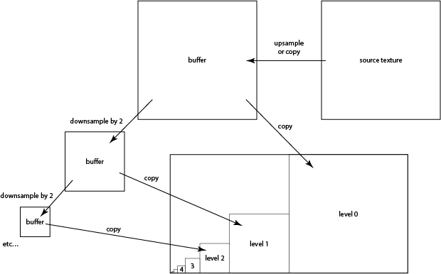
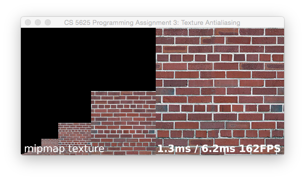
Using the D key you can get the framework to show you this buffer. The result should look something like this, for the brick-256 texture:
Sampling from the mipmap. To complete this part, implement basic mipmapping. This means adding the MODE_TRILINEAR mode to your texture filtering shader, doing a linear interpolaton in the mipmap for each of two levels and blending them based on the desired level of detail. In this section we outline a process for going through this somewhat tricky implementation.
1. Sample from a fixed mipmap level. Start by using a single hardcoded level, to make sure you can successfully bilinearly interpolate from each of the mipmap levels. From left to right, level hardcoded to 0 and 2 for the brick-256 texture:
Note that this scene requires GL_REPEAT style texture wrapping: the texture coordinates on the plane run from 0.0 to 25.0 on each axis. But this mode is not supported for rectangle textures (and it wouldn't solve the problem anyway, since our tiles are smaller than the texture). Your shader will have to explicitly wrap the texture coordinates, or you will just get one copy of the brick texture, way off in a corner of the world.
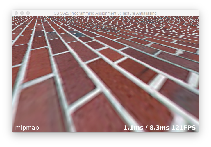
2. Sample from the appropriate mipmap level. Once you can sample from a hardcoded level, compute the mipmap level using the same derivatives you used to implement the supersampling mode, using the formula recommended by Williams in the paper referenced above. Then linearly interpolate between the integer levels on either side of the real-number mipmap level you compute. The result should look comparable to OpenGL's hardware mipmapping result (use the O key to flip back and forth):
though the exact appearance of textures using the built-in mipmapping will differ slightly from system to system depending on the filters used to build the hierarchy.
Details, details, … Your images will not yet look quite like this; you'll notice there are some artifacts along the seams between tiles. Why? How can you fix them without killing performance? Go ahead and fix them so there are no major seams (though a discontinuity is OK—but it's simple enough to remove that also). Hint: in our implementation, the mipmap buffer for a 256 by 256 texture is actually 530 by 256, and this version is what's shown in the image above.
Task 3: Anisotropic Texture Filtering
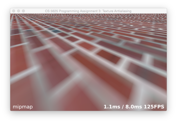
The mipmap is nice and fast, and it does get rid of the artifacts, but it blurs way too much in the distance. In this last section we will improve things by implementing an anisotropic filtering method described in the following paper:
J. McCormack, R. Perry, K. Farkas, and N. Jouppi, “Feline: Fast Elliptical Lines for Anisotropic Texture Mapping,” SIGGRAPH 1999.The main idea here is to average several lookups computed using your trilinear mipmapping code, with the lookup points positioned along the major axis of the ellipse defined by the texture coordinate derivatives.
Implementing anisotropic filtering is simple in principle, given your working mipmap implementation—though there are a lot of details to get right. From the formulas in the paper, using the derivatives given to you by dFdx and dFdy, compute the minor and major axis lengths of the filter footprint and the major axis direction. Select the mipmap level using the minor axis length, and make several lookups distributed along the major axis. When computing the weights for each of these lookups (or “probes” as the paper calls them), use a Gaussian function with α=2. The paper recommends 5 probes, but that was for slower hardware; if you want to match what your built-in graphics does, you'll want 8, 16, or 32.
You may compute the axes of the ellipse using either the trigonomentric fomulas that the authors describe in section 3.1, or using the Texram ellipse axis approximations described in section 3.2. Or you can use the eigenvalue approach sketched in lecture. If you choose to use the trigonometric formulas, be aware that glsl has two modes for the builtin atan function; the first, atan(y/x), takes in a single argument and returns an angle in the range [−π2,π2], and the second, atan(y,x), is the equivalent of Java's atan2 method and returns an angle in the range [−π,π].
For those interested in the math behind the formulas, David Eberly's explanation from his Geometric Tools series is excellent:
D. Eberly, “Information About Ellipses,” geometrictools.com.
Sections 3.2 and 3.3 describe further optimizations, including lookup tables and optimizing parameters. Feel free to implement these parts, but only the method described in Section 3.1 is required for this assignment.
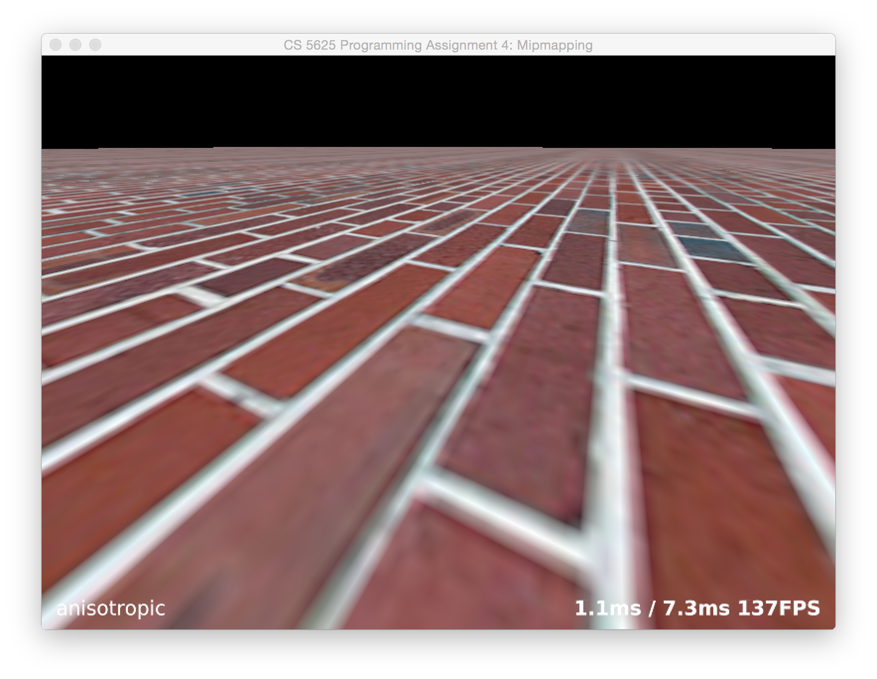
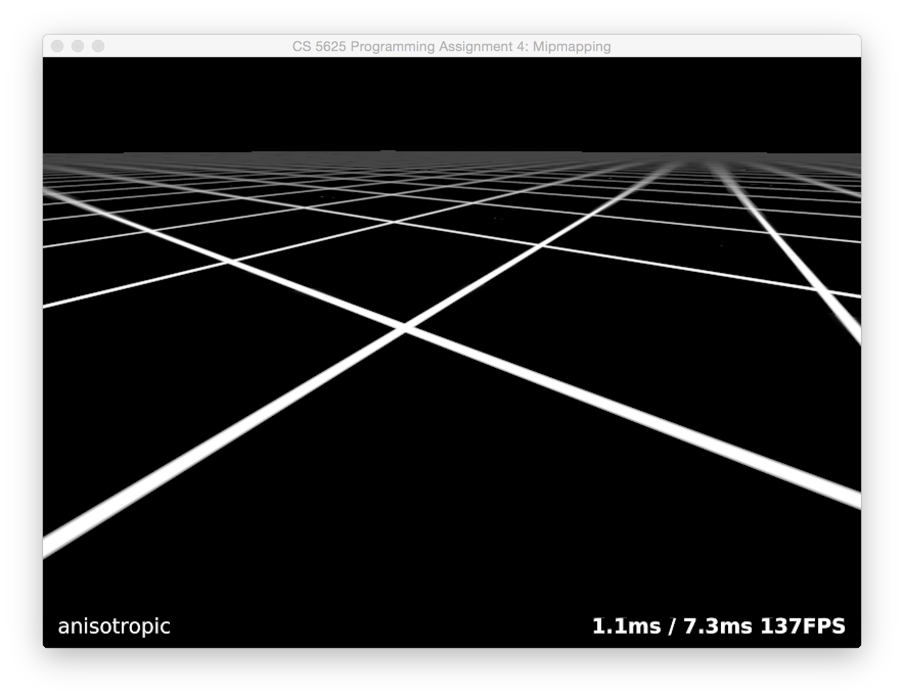
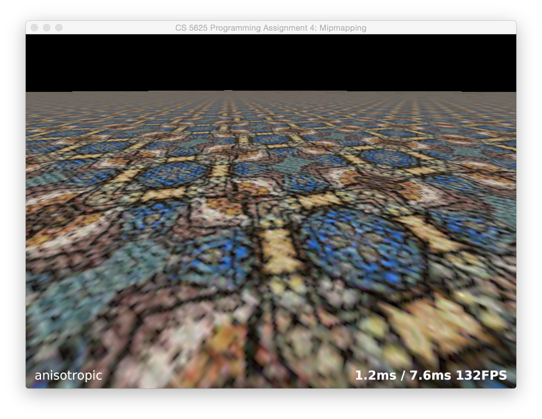
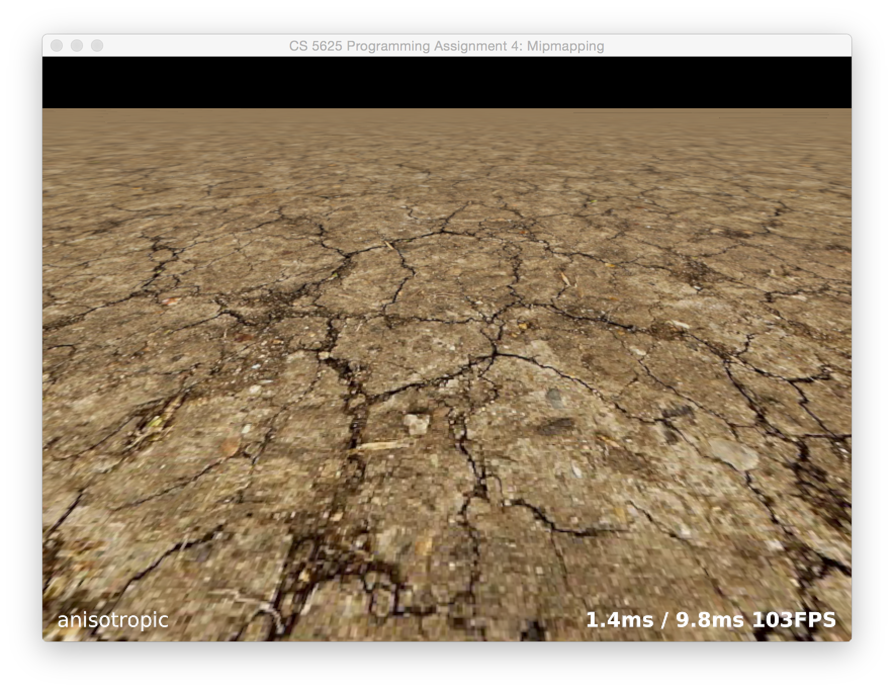
If you've implemented this task correctly, you should be able to see a major improvement over regular mipmapping. Increasing the maximum number of probes should further increase the quality, and you should be able to approximate your system's anisotropic shading (or beat it, on lower-end hardware) with enough probes. Below are some results from our Feline implementation:
Mode Keys
- b: nearest-neighbor sampling
- s: supersampling
- m: mipmap with trilinear interpolation
- a: mipmap with anisotropic filtering
- d: display the mipmap you computed
- o: turning on OpenGL-version (only works with box, mipmap, and anisotropic modes)
- ->: use next texture
- <-: use previous texture