
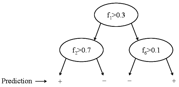
Binary decision tree. Only labels are stored.
Let us return to the k-nearest neighbor classifier. In low dimensions it is actually quite powerful: It can learn non-linear decision boundaries and naturally can handle multi-class problems. There are however a few catches: kNN uses a lot of storage (as we are required to store the entire training data), the more training data we have the slower it becomes during testing (as we need to compute distances to all training inputs), and finally we need a good distance metric.
Most data that is interesting has some inherent structure. In the k-NN case we make the assumption that similar inputs have similar neighbors. This would imply that data points of various classes are not randomly sprinkled across the space, but instead appear in clusters of more or less homogeneous class assignments. Although there are efficient data structures enable faster nearest neighbor search, it is important to remember that the ultimate goal of the classifier is simply to give an accurate prediction. Imagine a binary classification problem with positive and negative class labels. If you knew that a test point falls into a cluster of 1 million points with all positive label, you would know that its neighbors will be positive even before you compute the distances to each one of these million distances. It is therefore sufficient to simply know that the test point is an area where all neighbors are positive, its exact identity is irrelevant.
Decision trees are exploiting exactly that. Here, we do not store the training data, instead we use the training data to build a tree structure that recursively divides the space into regions with similar labels. The root node of the tree represents the entire data set. This set is then split roughly in half along one dimension by a simple threshold \(t\). All points that have a feature value \(\geq t\) fall into the right child node, all the others into the left child node. The threshold \(t\) and the dimension are chosen so that the resulting child nodes are purer in terms of class membership. Ideally all positive points fall into one child node and all negative points in the other. If this is the case, the tree is done. If not, the leaf nodes are again split until eventually all leaves are pure (i.e. all its data points contain the same label) or cannot be split any further (in the rare case with two identical points of different labels).
Decision trees have several nice advantages over nearest neighbor algorithms: 1. once the tree is constructed, the training data does not need to be stored. Instead, we can simply store how many points of each label ended up in each leaf - typically these are pure so we just have to store the label of all points; 2. decision trees are very fast during test time, as test inputs simply need to traverse down the tree to a leaf - the prediction is the majority label of the leaf; 3. decision trees require no metric because the splits are based on feature thresholds and not distances.
New goal: Build a tree that is:Binary decision tree. Only labels are stored.
Gini impurity of a tree: \[G^T(S)=\frac{\left | S_L \right |}{\left | S \right |}G^T(S_L)+\frac{\left | S_R \right |}{\left | S \right |}G^T(S_R)\] where: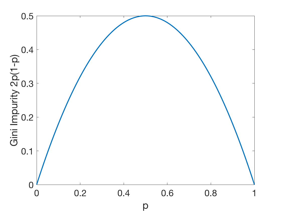
Fig: The Gini Impurity Function in the binary case reaches its maximum at \(p=0.5\).
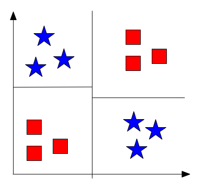
Fig 4: Example XOR
\[L(S)=\frac{1}{|S|}\sum_{(x,y)\in S}(y-\bar{y}_S)^2 \leftarrow\textrm{Average squared difference from average label}\] \[\textrm{where }\bar{y}_S=\frac{1}{|S|}\sum_{(x,y)\in S}y\leftarrow\textrm{Average label}\] At leaves, predict \(\bar{y}_S\). Finding best split only costs \(O(n\log n)\).
CART summary:
Fig: CART

Fig: ID3-trees are prone to overfitting as the tree depth increases. The left plot shows the learned decision boundary of a binary data set drawn from two Gaussian distributions. The right plot shows the testing and training errors with increasing tree depth.
So far we have introduced a variety of algorithms. One can categorize these into different families, such as generative vs. discriminative, or probabilistic vs. non-probabilistic. Here we will introduce another one, parametric vs. non-parametric.
A parametric algorithm is one that has a constant set of parameters, which is independent of the number of training samples. You can think of it as the amount of much space you need to store the trained classifier. An examples for a parametric algorithm is the Perceptron algorithm, or logistic regression. Their parameters consist of \(\mathbf{w},b\), which define the separating hyperplane. The dimension of \(\mathbf{w}\) depends of the dimension of the training data, but not on how many training samples you use for training.
In contrast, the number of parameters of a non-parametric algorithm scales as a function of the training samples. An example of a non-parametric algorithm is the \(k\)-Nearest Neighbors classifier. Here, during "training" we store the entire training data -- so the parameters that we learn are identical to the training set and the number of parameters (/the storage we require) grows linearly with the training set size.
An interesting edge case is kernel-SVM. Here it depends very much which kernel we are using. E.g. linear SVMs are parametric (for the same reason as the Perceptron or logistic regression). So if the kernel is linear the algorithm is clearly parametric. However, if we use an RBF kernel then we cannot represent the classifier of a hyper-plane of finite dimensions. Instead we have to store the support vectors and their corresponding dual variables \(\alpha_i\) -- the number of which is a function of the data set size (and complexity). Hence, the kernel-SVM with an RBF kernel is non-parametric. A strange in-between case is the polynomial kernel. It represents a hyper-plane in an extremely high but still finite-dimensional space. So technically one could represent any solution of an SVM with a polynomial kernel as a hyperplane in an extremely high dimensional space with a fixed number of parameters, and the algorithm is therefore (technically) parametric. However, in practice this is not practical. Instead, it is almost always more economical to store the support vectors and their corresponding dual variables (just like with the RBF kernel). It therefore is technically parametric but for all means and purposes behaves like a non-parametric algorithm.
Decision Trees are also an interesting case. If they are trained to full depth they are non-parametric, as the depth of a decision tree scales as a function of the training data (in practice \(O(\log_2(n))\)). If we however limit the tree depth by a maximum value they become parametric (as an upper bound of the model size is now known prior to observing the training data).