KD Trees

Cornell CS 4/5780

Spring 2022

Old Recorded Lecture

Time Complexity of k-NN

Let's look at the time complexity of $k$ -NN. Suppose we are in a $d$ -dimensional space, and we have trained on $n$ data points. With the naive $k$ -NN setup we saw earlier in the semester, our learned "model" is just a memorization of all the points in the training set, so our time complexity for training is $O (d n)$ , since we need to copy the whole training set. When testing, we need to compute the distance between our new data point and all of the data points we trained on. Classifying one test input is also $O (d n)$ , since we need to pass through the whole saved training set to compute the distances. To achieve the best accuracy we can, we would like our training data set to be very large ( $n ≫ 0$ ), but this will become a serious bottleneck during test time.

Previously, we looked at a lot of linear-model-based machine learning methods that avoid this problem by having a parameterized hypothesis class with fixed parameter dimension $d$ (i.e. $w \in R^{d}$ ) such that predictions take $O (d)$ time to make. But we also saw that this can limit the models we learn. Sometimes, we really want $k$ -NN behavior—not a linear model or even a kernel model—but we also want it to scale nicely to large datasets.

Goal: Can we make k-NN faster during testing?

We can do it—if we use clever data structures.

A thought experiment

Suppose I want to do 7-NN on a large dataset $D$ that is split up into two roughly-equally-sized portions, each possessed by one of my colleagues Alice and Bob. That is, $D = D_{Alice} \cup D_{Bob}$ . One way I can do this is the following. Given a test point $x$ , I ask Alice to run 7-NN for $x$ on her dataset. Then I ask Bob to run 7-NN for $x$ on his dataset. Then I find the seven nearest neighbors from among the fourteen returned by Alice and Bob.

Now, suppose that the 7th-nearest neighbor returned by Alice is at a distance 1 from $x$ . And when I look at the closest neighbor returned by Bob, I see it's at a distance 3 from $x$ . Do I even need to evaluate the other neighbors returned by Bob? No! They're all going to be further away than Alice's neighbors.

Imagine that Alice and Bob have their datasets stored such that sometimes they can give me a lower bound on the distance from $x$ to its nearest neighbor in their dataset—in much less time than it would require to run the full $k$ -NN search. Then a sequence of events like the following could occur:

Given $x$ , I ask Alice for a lower-bound on its distance-to-nearest-neighbor in her dataset. Alice outputs 0, a trivial lower bound.
I ask Bob for a lower-bound on $x$ 's distance-to-nearest-neighbor in his dataset. Bob outputs 2, a non-trivial lower bound.
I ask Alice to run 7-NN for $x$ on her dataset. Alice outputs 7 points, where the furthest one away from $x$ is at a distance 1.
I don't need to ask Bob to run 7-NN on his dataset, since I know Alice's neighbors are all going to be closer than anything in Bob's dataset.

Compared with the naive algorithm, I've saved the compute cost of processing Bob's dataset. This ability to save work with a lower bound on the distance to a set of points is what underlies the KD-tree datastructure.

k-Dimensional Trees

The general idea of KD-trees is to partition the feature space and search it cleverly rather than by brute force. Those of you who have taken CS4/5700 may recognize these ideas we're about to cover as similar to those used in search algorithms in AI, such as A* search. The plan is to create a data structure that enables us to "discard" (i.e. rule out as being one of the $k$ nearest neighbors) lots of data points in a single step because we can prove they are all further away than some $k$ points we've already found.

We partition the following way:

Divide your data into two halves, e.g. left and right, along one feature.
For each training input, remember the half it lies in.

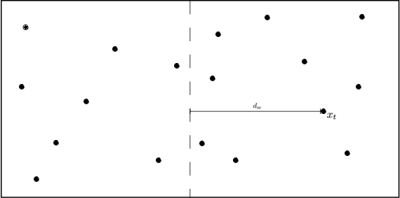
How can this partitioning speed up testing? Let's think about it for the 1-NN case.

Identify which side the test point lies in, e.g. the right side.
Find the nearest neighbor $x_{NN}^{R}$ of $x_{t}$ in the same side. The $R$ denotes that our nearest neighbor is also on the right side.
Compute the distance between $x_{y}$ and the dividing "wall". Denote this as $d_{w}$ .
If $d_{w} > d (x_{t}, x_{NN}^{R})$ you are done, and we get a 2x speedup.
Otherwise, we need to proceed to search the left-side partition.

Fig: Partitioning the feature space.

In other words: if the distance to the partition is larger than the distance to our closest neighbor, we know that none of the data points inside that partition can be closer. We can avoid computing the distance to any of the points in that entire partition.

We can prove this formally with the triangle inequality. (See Figure 2 for an illustration.)
Let $d (x_{t}, x)$ denote the distance between our test point $x_{t}$ and a candidate $x$ . We know that $x$ lies on the other side of the wall, so this distance is dissected into two parts $d (x_{t}, x) = d_{1} + d_{2}$ , where $d_{1}$ is the part of the distance on $x_{t}^{'} s$ side of the wall and $d_{2}$ is the part of the distance on $x^{'} s$ side of the wall. Also let $d_{w}$ denote the shortest distance from $x_{t}$ to the wall. We know that $d_{1} > d_{w}$ and therefore it follows that $d (x_{t}, x) = d_{1} + d_{2} \geq d_{w} + d_{2} \geq d_{w} .$ This implies that if $d_{w}$ is already larger than the distance to the current best candidate point for the nearest neighbor, we can safely discard $x$ as a candidate.

Fig 2: The bounding of the distance between ${\vec{x}}_{t}$ and $\vec{x}$ with KD-trees and Ball trees (here $\vec{x}$ is drawn twice, once for each setting). The distance can be dissected into two components $d ({\vec{x}}_{t}, \vec{x}) = d_{1} + d_{2}$ , where $d_{1}$ is the outside ball/box component and $d_{2}$ the component inside the ball/box. In both cases $d_{1}$ can be lower bounded by the distance to the wall, $d_{w}$ , or ball, $d_{b}$ , respectively i.e. $d ({\vec{x}}_{t}, \vec{x}) = d_{1} + d_{2} \geq d_{w} + d_{2} \geq d_{w}$ .

Quiz: Construct a case where this does not work.

KD-tree data structure

Fig: The partitioned feature space with corresponding KD-tree.

Tree Construction:

Split data recursively in half on exactly one feature.
Rotate through features.

When rotating through features, a good heuristic is to pick the feature with maximum variance.

Example:

Which partitions can be pruned?
Which must be searched and in what order?
Pros:

Exact.
Easy to build.

Cons:

Curse of Dimensionality makes KD-Trees ineffective for higher number of dimensions.
All splits are axis aligned.

Approximation: Limit search to

m

leafs only.

Ball-trees

Similar to KD-trees, but instead of boxes use hyper-spheres (balls). (See Figure 2 for an illustration.)
As before we can dissect the distance and use the triangular inequality

d (x_{t}, x) = d_{1} + d_{2} \geq d_{b} + d_{2} \geq d_{b}

If the distance to the ball,

d_{b}

, is larger than distance to the currently closest neighbor, we can safely ignore the ball and all points within.
The ball structure allows us to partition the data along an underlying manifold that our points are on, instead of repeatedly dissecting the entire feature space (as in KD-Trees).

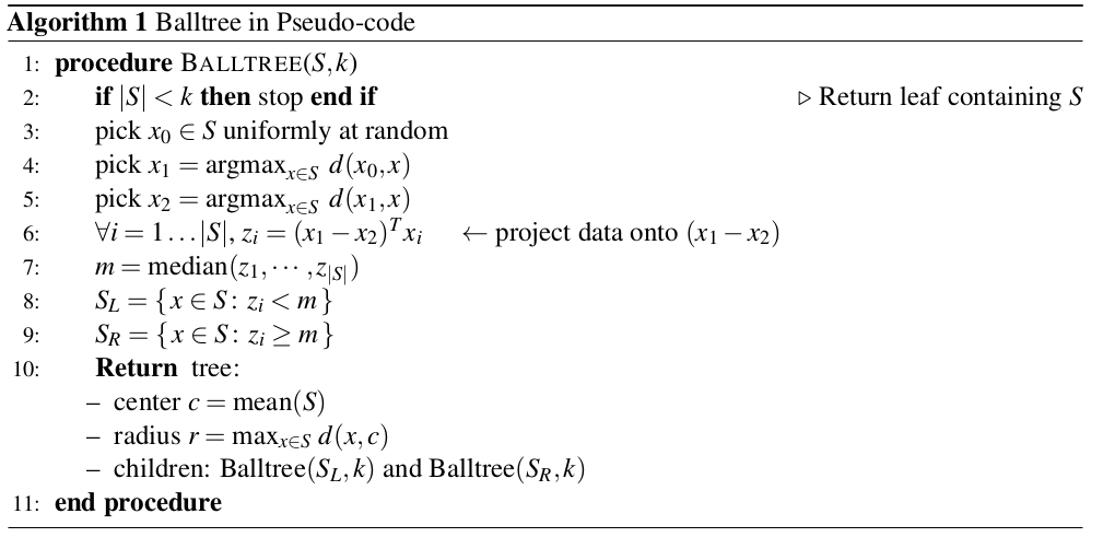
Ball-tree Construction

Input: set

S

n = | S |

k

Note: Steps 3 & 4 pick the direction with a large spread (

x_{1} - x_{2}

)

Ball-Tree Use

Same as KD-Trees
Slower than KD-Trees in low dimensions (

d \leq 3

) but a lot faster in high dimensions. Both are affected by the curse of dimensionality, but Ball-trees tend to still work if data exhibits local structure (e.g. lies on a low-dimensional manifold).

Summary

$k$ -NN is slow during testing because it does a lot of unecessary work.
KD-trees partition the feature space so we can rule out whole partitions that are further away than our closest $k$ neighbors. However, the splits are axis aligned which does not extend well to higher dimensions.
Ball-trees partition the manifold the points are on, as opposed to the whole space. This allows it to perform much better in higher dimensions.