Lecture 12: Bias-Variance Tradeoff

previous
next


As usual, we are given a dataset $D = \{(\mathbf{x}_1, y_1), \dots, (\mathbf{x}_n,y_n)\}$, drawn i.i.d. from some distribution $P(X,Y)$. Throughout this lecture we assume a regression setting, i.e. $y \in \mathbb{R}$. In this lecture we will decompose the generalization error of a classifier into three rather interpretable terms. Before we do that, let us consider that for any given input $\mathbf{x}$ there might not exist a unique label $y$. For example, if your vector $\mathbf{x}$ describes features of house (e.g. #bedrooms, square footage, ...) and the label $y$ its price, you could imagine two houses with identical description selling for different prices. So for any given feature vector $\mathbf{x}$, there is a distribution over possible labels. We therefore define the following, which will come in useful later on:
Expected Label (given $\mathbf{x} \in \mathbb{R}^d$): \[ \bar{y}(\mathbf{x}) = E_{y \vert \mathbf{x}} \left[Y\right] = \int\limits_y y \, \Pr(y \vert \mathbf{x}) \partial y. \] The expected label denotes the label you would expect to obtain, given a feature vector $\mathbf{x}$.
Alright, so we draw our training set $D$, consisting of $n$ inputs, i.i.d. from the distribution $P$. As a second step we typically call some machine learning algorithm $\mathcal{A}$ on this data set to learn a hypothesis (aka classifier). Formally, we denote this process as $h_D = \mathcal{A}(D)$.
For a given $h_D$, learned on data set $D$ with algorithm $\mathcal{A}$, we can compute the generalization error (as measured in squared loss) as follows:

Expected Test Error (given $h_D$):
\[ E_{(\mathbf{x},y) \sim P} \left[ \left(h_D (\mathbf{x}) - y \right)^2 \right] = \int\limits_x \! \! \int\limits_y \left( h_D(\mathbf{x}) - y\right)^2 \Pr(\mathbf{x},y) \partial y \partial \mathbf{x}. \] Note that one can use other loss functions. We use squared loss because it has nice mathematical properties, and it is also the most common loss function.
The previous statement is true for a given training set $D$. However, remember that $D$ itself is drawn from $P^n$, and is therefore a random variable. Further, $h_D$ is a function of $D$, and is therefore also a random variable. And we can of course compute its expectation:

Expected Classifier (given $\mathcal{A}$): \[ \bar{h} = E_{D \sim P^n} \left[ h_D \right] = \int\limits_D h_D \Pr(D) \partial D \] where $\Pr(D)$ is the probability of drawing $D$ from $P^n$. Here, $\bar{h}$ is a weighted average over functions.
We can also use the fact that $h_D$ is a random variable to compute the expected test error only given $\mathcal{A}$, taking the expectation also over $D$.

Expected Test Error (given $\mathcal{A}$): \begin{equation*} E_{\substack{(\mathbf{x},y) \sim P\\ D \sim P^n}} \left[\left(h_{D}(\mathbf{x}) - y\right)^{2}\right] = \int_{D} \int_{\mathbf{x}} \int_{y} \left( h_{D}(\mathbf{x}) - y\right)^{2} \mathrm{P}(\mathbf{x},y) \mathrm{P}(D) \partial \mathbf{x} \partial y \partial D \end{equation*} To be clear, $D$ is our training points and the $(\mathbf{x},y)$ pairs are the test points.
We are interested in exactly this expression, because it evaluates the quality of a machine learning algorithm $\mathcal{A}$ with respect to a data distribution $P(X,Y)$. In the following we will show that this expression decomposes into three meaningful terms.

Decomposition of Expected Test Error

\begin{align} E_{\mathbf{x},y,D}\left[\left[h_{D}(\mathbf{x}) - y\right]^{2}\right] &= E_{\mathbf{x},y,D}\left[\left[\left(h_{D}(\mathbf{x}) - \bar{h}(\mathbf{x})\right) + \left(\bar{h}(\mathbf{x}) - y\right)\right]^{2}\right] \nonumber \\ &= E_{\mathbf{x}, D}\left[(\bar{h}_{D}(\mathbf{x}) - \bar{h}(\mathbf{x}))^{2}\right] + 2 \mathrm{\;} E_{\mathbf{x}, y, D} \left[\left(h_{D}(\mathbf{x}) - \bar{h}(\mathbf{x})\right)\left(\bar{h}(\mathbf{x}) - y\right)\right] + E_{\mathbf{x}, y} \left[\left(\bar{h}(\mathbf{x}) - y\right)^{2}\right] \label{eq:eq1} \end{align} The middle term of the above equation is $0$ as we show below \begin{align*} E_{\mathbf{x}, y, D} \left[\left(h_{D}(\mathbf{x}) - \bar{h}(\mathbf{x})\right) \left(\bar{h}(\mathbf{x}) - y\right)\right] &= E_{\mathbf{x}, y} \left[E_{D} \left[ h_{D}(\mathbf{x}) - \bar{h}(\mathbf{x})\right] \left(\bar{h}(\mathbf{x}) - y\right) \right] \\ &= E_{\mathbf{x}, y} \left[ \left( E_{D} \left[ h_{D}(\mathbf{x}) \right] - \bar{h}(\mathbf{x}) \right) \left(\bar{h}(\mathbf{x}) - y \right)\right] \\ &= E_{\mathbf{x}, y} \left[ \left(\bar{h}(\mathbf{x}) - \bar{h}(\mathbf{x}) \right) \left(\bar{h}(\mathbf{x}) - y \right)\right] \\ &= E_{\mathbf{x}, y} \left[ 0 \right] \\ &= 0 \end{align*} Returning to the earlier expression, we're left with the variance and another term \begin{equation} E_{\mathbf{x}, y, D} \left[ \left( h_{D}(\mathbf{x}) - y \right)^{2} \right] = \underbrace{E_{\mathbf{x}, D} \left[ \left(h_{D}(\mathbf{x}) - \bar{h}(\mathbf{x}) \right)^{2} \right]}_\mathrm{Variance} + E_{\mathbf{x}, y}\left[ \left( \bar{h}(\mathbf{x}) - y \right)^{2} \right] \label{eq:eq2} \end{equation} We can break down the second term in the above equation as follows: \begin{align} E_{\mathbf{x}, y} \left[ \left(\bar{h}(\mathbf{x}) - y \right)^{2}\right] &= E_{\mathbf{x}, y} \left[ \left(\bar{h}(\mathbf{x}) -\bar y(\mathbf{x}) )+(\bar y(\mathbf{x}) - y \right)^{2}\right] \\ &=\underbrace{E_{\mathbf{x}, y} \left[\left(\bar{y}(\mathbf{x}) - y\right)^{2}\right]}_\mathrm{Noise} + \underbrace{E_{\mathbf{x}} \left[\left(\bar{h}(\mathbf{x}) - \bar{y}(\mathbf{x})\right)^{2}\right]}_\mathrm{Bias^2} + 2 \mathrm{\;} E_{\mathbf{x}, y} \left[ \left(\bar{h}(\mathbf{x}) - \bar{y}(\mathbf{x})\right)\left(\bar{y}(\mathbf{x}) - y\right)\right] \label{eq:eq3} \end{align} The third term in the equation above is $0$, as we show below \begin{align*} E_{\mathbf{x}, y} \left[\left(\bar{h}(\mathbf{x}) - \bar{y}(\mathbf{x})\right)\left(\bar{y}(\mathbf{x}) - y\right)\right] &= E_{\mathbf{x}}\left[E_{y \mid \mathbf{x}} \left[\bar{y}(\mathbf{x}) - y \right] \left(\bar{h}(\mathbf{x}) - \bar{y}(\mathbf{x}) \right) \right] \\ &= E_{\mathbf{x}} \left[ E_{y \mid \mathbf{x}} \left[ \bar{y}(\mathbf{x}) - y\right] \left(\bar{h}(\mathbf{x}) - \bar{y}(\mathbf{x})\right)\right] \\ &= E_{\mathbf{x}} \left[ \left( \bar{y}(\mathbf{x}) - E_{y \mid \mathbf{x}} \left [ y \right]\right) \left(\bar{h}(\mathbf{x}) - \bar{y}(\mathbf{x})\right)\right] \\ &= E_{\mathbf{x}} \left[ \left( \bar{y}(\mathbf{x}) - \bar{y}(\mathbf{x}) \right) \left(\bar{h}(\mathbf{x}) - \bar{y}(\mathbf{x})\right)\right] \\ &= E_{\mathbf{x}} \left[ 0 \right] \\ &= 0 \end{align*} This gives us the decomposition of expected test error as follows \begin{equation*} \underbrace{E_{\mathbf{x}, y, D} \left[\left(h_{D}(\mathbf{x}) - y\right)^{2}\right]}_\mathrm{Expected\;Test\;Error} = \underbrace{E_{\mathbf{x}, D}\left[\left(h_{D}(\mathbf{x}) - \bar{h}(\mathbf{x})\right)^{2}\right]}_\mathrm{Variance} + \underbrace{E_{\mathbf{x}, y}\left[\left(\bar{y}(\mathbf{x}) - y\right)^{2}\right]}_\mathrm{Noise} + \underbrace{E_{\mathbf{x}}\left[\left(\bar{h}(\mathbf{x}) - \bar{y}(\mathbf{x})\right)^{2}\right]}_\mathrm{Bias^2} \end{equation*} Variance: Captures how much your classifier changes if you train on a different training set. How "over-specialized" is your classifier to a particular training set (overfitting)? If we have the best possible model for our training data, how far off are we from the average classifier?

Bias: What is the inherent error that you obtain from your classifier even with infinite training data? This is due to your classifier being "biased" to a particular kind of solution (e.g. linear classifier). In other words, bias is inherent to your model.

Noise: How big is the data-intrinsic noise? This error measures ambiguity due to your data distribution and feature representation. You can never beat this, it is an aspect of the data.

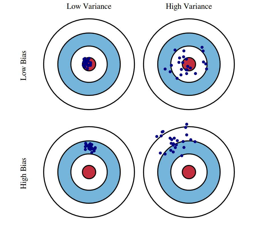
Fig 1: Graphical illustration of bias and variance.
Source: http://scott.fortmann-roe.com/docs/BiasVariance.html

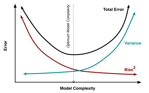
Fig 2: The variation of Bias and Variance with the model complexity. This is similar to the concept of overfitting and underfitting. More complex models overfit while the simplest models underfit.
Source: http://scott.fortmann-roe.com/docs/BiasVariance.html

Detecting High Bias and High Variance

If a classifier is under-performing (e.g. if the test or training error is too high), there are several ways to improve performance. To find out which of these many techniques is the right one for the situation, the first step is to determine the root of the problem.

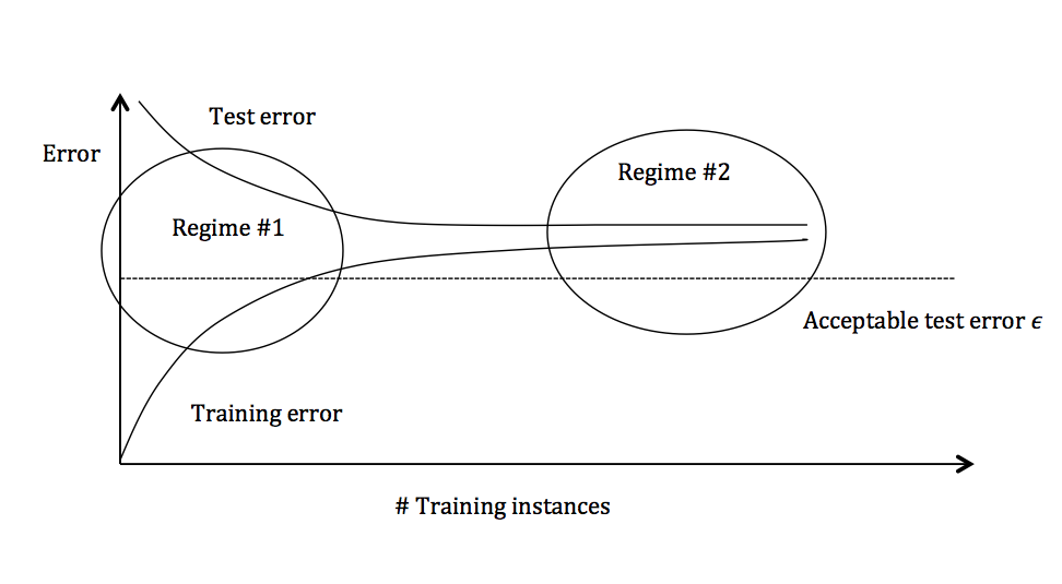
Figure 3: Test and training error as the number of training instances increases.

The graph above plots the training error and the test error and can be divided into two overarching regimes. In the first regime (on the left side of the graph), training error is below the desired error threshold (denoted by $\epsilon$), but test error is significantly higher. In the second regime (on the right side of the graph), test error is remarkably close to training error, but both are above the desired tolerance of $\epsilon$.

Regime 1 (High Variance)

In the first regime, the cause of the poor performance is high variance.

Symptoms:

  1. Training error is much lower than test error
  2. Training error is lower than $\epsilon$
  3. Test error is above $\epsilon$

Remedies:

Regime 2 (High Bias)

Unlike the first regime, the second regime indicates high bias: the model being used is not robust enough to produce an accurate prediction.

Symptoms:

  1. Training error is higher than $\epsilon$

Remedies: