Project 5: Bias Variance Trade-off

"All of us show bias when it comes to what information we take in.
We typically focus on anything that agrees with the outcome we want."
--Noreena Hertz

Introduction

Recall that the squared error can be decomposed into bias, variance and noise: $$ \underbrace{\mathbb{E}[(h_D(x) - y)^2]}_\mathrm{Error} = \underbrace{\mathbb{E}[(h_D(x)-\bar{h}(x))^2]}_\mathrm{Variance} + \underbrace{\mathbb{E}[(\bar{h}(x)-\bar{y}(x))^2]}_\mathrm{Bias} + \underbrace{\mathbb{E}[(\bar{y}(x)-y(x))^2]}_\mathrm{Noise}\nonumber $$ We will now create a data set for which we can approximately compute this decomposition. The function toydata.m generates a binary data set with class $1$ and $2$. Both are sampled from Gaussian distributions: \begin{equation} p(\vec x|y=1)\sim {\mathcal{N}}(0,{I}) \textrm { and } p(\vec x|y=2)\sim {\mathcal{N}}(\mu_2,{I}),\label{eq:gaussian} \end{equation} where $\mu_2=[2;2]^\top$ (the global variable OFFSET $\!=\!2$ regulates these values: $\mu_2=[$OFFSET $;$ OFFSET$]^\top$).

Computing noise, bias and variance

You will need to edit four functions: computeybar.m, computehbar.m, computevariance.m and biasvariancedemo.m. First take a look at biasvariancedemo.m and make sure you understand where each function should be called and how they contribute to the Bias/Variance/Noise decomposition.

(a) Noise: First we focus on the noise. For this, you need to compute $\bar y(\vec x)$ in computeybar.m. With the equations, $p(\vec x|y=1)\sim {\mathcal{N}}(0,{I}) \textrm { and } p(\vec x|y=2)\sim {\mathcal{N}}(\mu_2,{I})$, you can compute the probability $p(\vec x|y)$. Then use Bayes rule to compute $p(y|\vec x)$.

Note: You may want to use the function normpdf, which is defined for you in computeybar.m.

With the help of computeybar.m you can now compute the "noise" variable within biasvariancedemo.m.

(b) Bias: For the bias, you will need $\bar{h}$. Although we cannot compute the expected value $\bar h\!=\!\mathbb{E}[h]$, we can approximate it by training many $h_D$ and averaging their predictions. Edit the file computehbar.m: average over NMODELS different $h_D$, each trained on a different data set of Nsmall inputs drawn from the same distribution. Feel free to call toydata.m to obtain more data sets.

Note: $h_D$ is defined for you in kregression.m. It's kernelized ridge regression with kernel width $\sigma$ and regularization constant $\lambda$.

With the help of computehbar.m you can now compute the "bias" variable within biasvariancedemo.m.

(c) Variance: Finally, to compute the variance, we need to compute the term $\mathbb{E}[(h_D-\bar{h})^2]$. Once again, we can approximate this term by averaging over NMODELS models. Edit the file computevariance.m.

With the help of computevariance.m you can now compute the "variance" variable within biasvariancedemo.m.

If you did everything correctly and call biasvariancedemo.m, you should see how the error decomposes (roughly) into bias, variance and noise when regularization constant $\lambda$ increases.

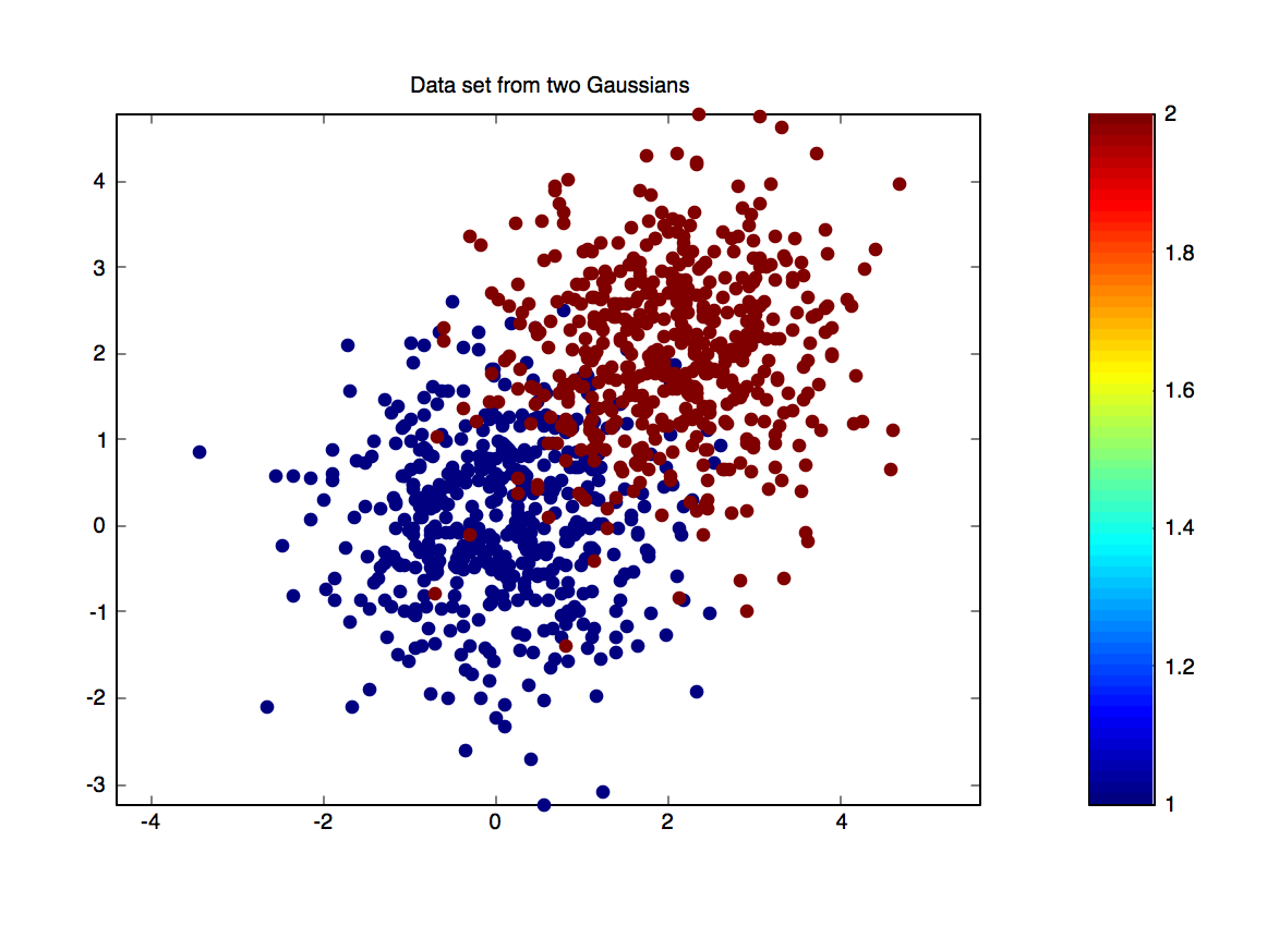
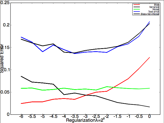
Left: a plot of the binary data set with means $\vec{0}$ and $[2,2]^\top$. Right: The decomposition of test error into bias, variance and noise.

Note

hw05tests.m tests if your implementations are correct.

When computing the bias and variance, you approximate the results by training many $h_D$. We set NMODELS=1000 and use some thresholds to test if your functions' results are correct. Unfortunately, as a result of this randomness, there is still a small chance that you will fail some test cases, even though your implementations are correct.

If you can pass all the tests most of the times locally, then you are fine. In this case, if the autograder says your accuracy is not 100%, just commit the code again.

There is no competition this time.