Lecture 16: Gaussian Process
Gaussian Distribution
We first review the definition and properties of Gaussian distribution:
A Gaussian random variable $X\sim \mathcal{N}(\mu,\Sigma)$, where $\mu$ is the mean and $\Sigma$ is the covariance matrix has the following probability density function:
$$P(x;\mu,\Sigma)=\frac{1}{(2\pi)^{\frac{d}{2}}|\Sigma|}e^{-\frac{1}{2}((x-\mu)^\top \Sigma^{-1}(x-\mu)}$$
where $|\Sigma|$ is the determinant of $\Sigma$.
Gaussian distribution occurs very often in real life - probably because of the Central Limit Theorem. The CLT states that, given some conditions, the arithmetic mean of $m>0$ samples is approximately normal distributed - independent of the sample distribution.
Let Gaussian random variable $Y=\begin{pmatrix} Y_A\\ Y_B \end{pmatrix}$, mean $\mu=\begin{pmatrix} \mu_A\\ \mu_B \end{pmatrix}$ and covariance matrix $\Sigma=\begin{pmatrix} \Sigma_{AA}, \Sigma_{AB} \\ \Sigma_{BA}, \Sigma_{BB} \end{pmatrix}$. We have the following properties:
1. Normalization: $\int_y p(y;\mu,\Sigma)dy=1$.
2. Marginalization: The marginal distribution $p(y_A)=\int_{y_B}p(y_A,y_B;\mu,\Sigma)dy_B$, and $y_A\sim \mathcal{N}(\mu_A,\Sigma_{AA})$; similarly, the marginal distribution $p(y_B)=\int_{y_A}p(y_A,y_B;\mu,\Sigma)dy_A$, and $y_B\sim \mathcal{N}(\mu_B,\Sigma_{BB})$.
3. Summation: If $Y\sim \mathcal{N}(\mu,\Sigma)$ and $Y'\sim \mathcal{N}(\mu',\Sigma')$, then $Y+Y'\sim \mathcal{N}(\mu+\mu',\Sigma+\Sigma')$.
4. Conditioning: The conditional distribution of $Y_A$ on $Y_B$ is also Gaussian. $p(y_A|y_B)=\frac{p(y_A,y_B;\mu,\Sigma)}{\int_{y_A}p(y_A,y_B;\mu,\Sigma)dy_A}$, and $Y_A|Y_B=y_b\sim \mathcal{N}(\mu_A+\Sigma_{AB}\Sigma_{BB}^{-1}(y_B-\mu_B),\Sigma_{AA}-\Sigma_{AB}\Sigma_{BB}^{-1}\Sigma_{BA}). $
How GPR works
We assume that, before we observe the training labels, the labels are drawn from Gaussian distribution:
$$
\begin{pmatrix}
Y_1\\
Y_2\\
\vdots\\
Y_n\\
Y_t
\end{pmatrix}
\sim \mathcal{N}(0,\Sigma)$$
Zero-mean is always possible by subtracting sample mean.
All training and test labels are drawn from an $(n+m)$-dimension Gaussian distribution, where $n$ is the number of training points, $m$ is the number of testing points. Note that, the real training labels, $y_1,...,y_n$, we observe are samples of $Y_1,...,Y_n$.
For now, without loss of generality, let us only consider $m=1$
test point.
$y_1$,$y_2$ are independent:
pic
$$\Sigma_{ij}=\Sigma_{ji}=0$$
$y_1$,$y_2$ are pos.correlated:
pic
$$\Sigma_{ij}=\Sigma_{ji}>0$$
Because of the conditioning properties of Gaussians, we obtain:
$$
P(y_+|y_1,y_2,\dots,y_n;\Sigma) ~ ~\text{is Gaussian.}
$$
Whether this distribution gives us meaningful distribution or not depends on how we choose the covariance matrix $\Sigma$. We consider the following properties of $\Sigma$:
1. $\Sigma_{ij}=E((Y_i-\mu_i)(Y_j-\mu_j))$.
2. $\Sigma$ is always positive semi-definite.
3. $\Sigma_{ii}=\text{Variance}(Y_i)$, thus $\Sigma_{ii}\geq 0$.
4. If $Y_i$ and $Y_j$ are very independent, i.e. $x_i$ is very different from $x_j$, then $\Sigma_{ij}=\Sigma_{ji}=0$.
5. If $x_i$ is similar to $x_j$, then $\Sigma_{ij}=\Sigma_{ji}>0$.
We can observe that this is very similar from the kernel matrix in SVMs. Therefore, we can simply let $\Sigma_{ij}=K(x_i,x_j)$. For example, if we use RBF kernel (aka ``squared exponential kernel''), then
\begin{equation}
\Sigma_{ij}=\tau e^\frac{-\|x_i-x_j\|^2}{\sigma^2}.
\end{equation}
If we use polynomial kernel, then $\Sigma_{ij}=\tau (1+x_i^\top x_j)^d$.
Thus, we can decompose $\Sigma$ as $\begin{pmatrix} K, K_t \\K_t^\top , K_{tt} \end{pmatrix}$, where $K$ is the training kernel matrix, $K_t$ is the training-testing kernel matrix, $K_t^\top $ is the testing-training kernel matrix and $K_{tt}$ is the testing kernel matrix. The conditional distribution of testing labels can be written as:
\begin{equation}
Y_t|(Y_1=y_1,...,Y_n=y_n,x_1,...,x_n,x_t)\sim \mathcal{N}(K_t^\top K^{-1}y,K_{tt}-K_t^\top K^{-1}K_t),
\end{equation}
where the kernel matrices $K_t, K_{tt}, K$ are functions of $x_1,\dots,x_n,x_t$.
Gaussian Process Regression has the following properties:
- GPs work very well for regression problems with small training data set sizes.
- GPs are awkward for classification (just use SVMs).
- Running time $O(n^3) \leftarrow $ matrix inversion (gets slow when $n\gg 0$).
Additive Gaussian Noise
In many applications the observed labels can be noisy. If we assume this noise is independent and zero-mean Gaussian, then we observe $\hat Y_i=Y_i+\epsilon_i$, where $Y_i$ is the true (unobserved) label and the noise is denoted by $\epsilon_i\sim \mathcal{N}(0,\sigma^2)$. In this case the new covariance matrix becomes $\hat\Sigma=\Sigma+\sigma^2\mathbf{I}$. We can derive this fact first for the off-diagonal terms where $i\neq j$
\begin{equation}
\hat\Sigma_{ij}=\mathbb{E}[(Y_i+\epsilon_i)(Y_j+\epsilon_j)]=\mathbb{E}[Y_iY_j]+\mathbb{E}[Y_i]\mathbb{E}[\epsilon_j]+\mathbb{E}[Y_j]\mathbb{E}[\epsilon_i]+\mathbb{E}[\epsilon_i]\mathbb{E}[\epsilon_j]=\mathbb{E}[Y_iY_j]=\Sigma_{ij},
\end{equation}
as $\mathbb{E}[\epsilon_i]=\mathbb{E}[\epsilon_j]=0$ and where we use the fact that $\epsilon_i$ is independent from all other random variables.
For the diagonal entries of $\Sigma$, i.e. the case where $i=j$, we obtain
\begin{equation}
\hat\Sigma_{ii}=\mathbb{E}[(Y_i+\epsilon_i)^2]=\mathbb{E}[Y_i^2]+2\mathbb{E}[Y_i]\mathbb{E}[\epsilon_i]+\mathbb{E}[\epsilon_i^2]=\mathbb{E}[Y_iY_j]+\mathbb{E}[\epsilon_i^2]=\Sigma_{ij}+\sigma^2,
\end{equation}
because $E[\epsilon_i^2]=\sigma^2$, which denotes the variance if $\epsilon_i$.
Plugging this updated covariance matrix into the Gaussian Process posterior distribution leads to
\begin{equation}
Y_t|(Y_1=y_1,...,Y_n=y_n,x_1,...,x_n)\sim \mathcal{N}(K_t^\top (K+\sigma^2 I)^{-1}y,K_{tt}+\sigma^2 I-K_t^\top (K+\sigma^2 I)^{-1}K_t).\label{eq:GP:withnoise}
\end{equation}
In practice the above equation is often more stable because the matrix $(K+\sigma^2 I)$ is always invertible of $\sigma^2$ is sufficiently large.
Bayesian Global Optimization
A nice applications of GP regression is Bayesian Global Optimization. Here, the goal is to optimize the hyper-parameters of a machine learning algorithm to do well on a fixed validation data set. Imagine you have $d$ hyper-parameters to tune, then your data set consists of $d-$dimensional vectors $x_i\in{\mathcal{R}}^d$, where each training point represents a particular hyper parameter setting and the labels $y_i\in{\mathcal R}$ represents the validation error.
Don't get confused, this time vectors $x_i$ correspond to hyperparameter settings and not data.
For example, in the case of an SVM with polynomial kernel you have two hyperparameters: the regularization constant $C$ (also often $\lambda$) and the polynomial power $p$. The first dimension of $x_i$ may correspond to a value for $C$ and the second dimension may correspond to a value of $p$.
Initially you run a few random settings and evaluate the classifier on the validation set. This gives you $x_1,\dots,x_m$ with labels $y_1,\dots,y_m$. You can now train a Gaussian Process to predict the validation error $y_t$ at any new hyperparameter setting $x_t$. In fact, you obtain a mean prediction $y_t=h(x_t)$ and its variance $v(x_t)$. If you have more time you can now explore a new point. The most promising point is the one with the lowest lower confidence bound, i.e.
\begin{equation}
argmin_{x_t} h(x_t)-\kappa\sqrt{v(x_t)}.
\end{equation}
The constant $\kappa>0$ trades off how much you want to explore points that may be good just because you are very uncertain (variance is high) or how much you want to exploit your knowledge about the current best point and refine the best settings found so far. A small $\kappa$ leads to more exploitation, whereas a large $\kappa$ explores new hyper-parameter settings more aggressively.
Algorithm:${\mathcal{A}},m,n,\kappa$
For $i$ = 1 to $m$
sample $x_i$ randomly e.g. sample uniformly within reasonable range
$y_i=\mathcal{A}(x_i)$ Compute validation error
EndFor
For $i$ = $m+1$ to $n$
Update kernel $K$ based on $x_1,\dots,x_{i-1}$
$x_i=argmin_{x_t} K_t^\top(K+\sigma^2 I)^{-1}y-\kappa\sqrt{K_{tt}+\sigma^2 I-K_t^\top (K+\sigma^2 I)^{-1}K_t}$
$y_i=\mathcal{A}(x_i)$ Compute validation error
Endfor
$i_{best}=argmin_{y_i}$ Find best hyper-parameter setting explored.
Return $x_{i_{best}}$
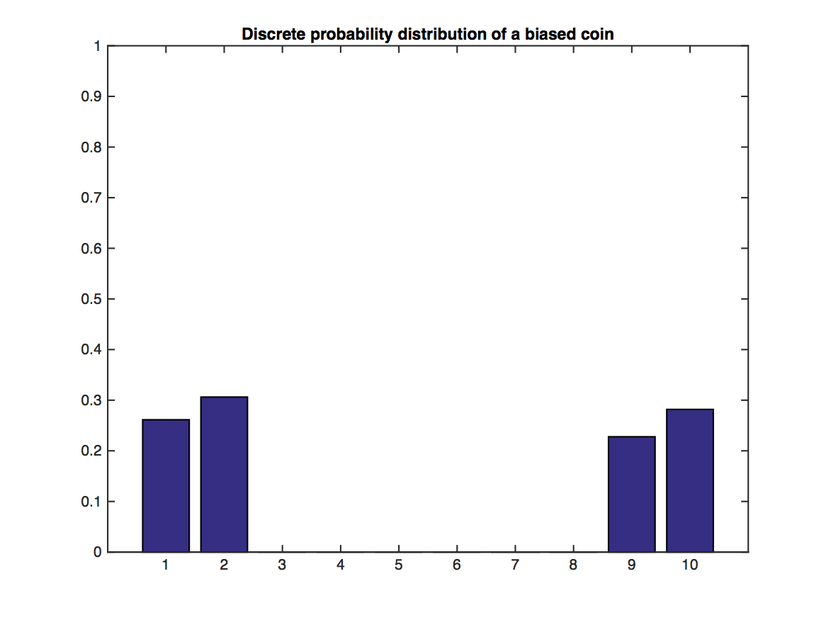
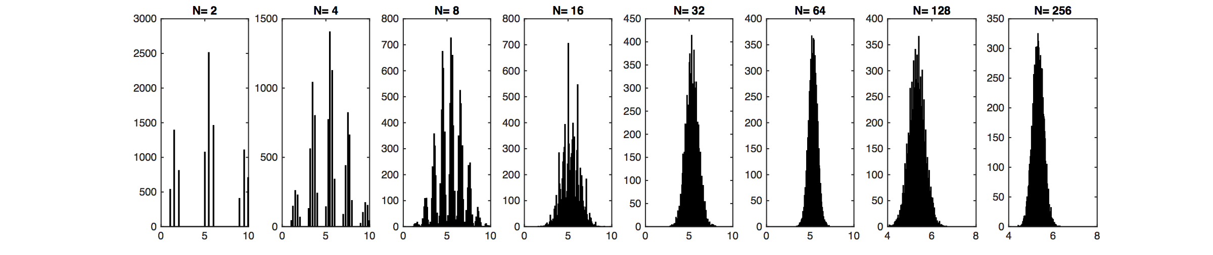
In the above graph, we try to make a distribution that is very ``non-Gaussian". However, the distribution of $m$ sample's mean, as we can observe, gets very ``Gaussian" as $m$ increases.

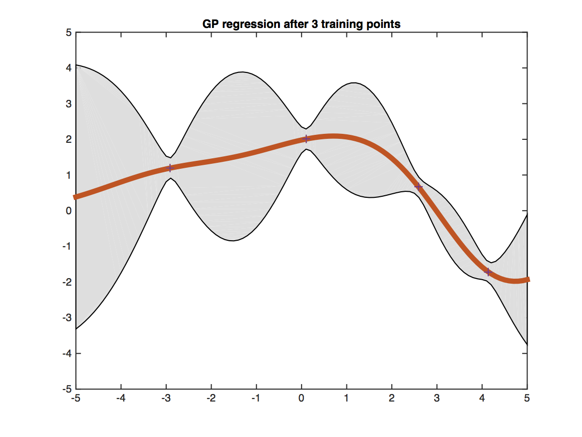
Testing points having more similar features with training points get more certain predictions.
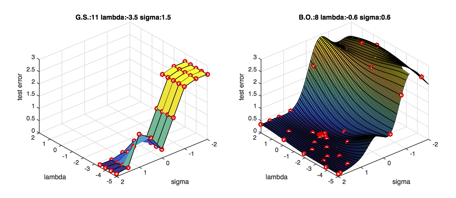
BO is much faster than grid search.