Lecture 12: Bias Variance Tradeoff

Lecture 12: Bias-Variance Tradeoff

As usual, we have a dataset

$D = \{(\mathbf{x}_1, y_1), \dots, (\mathbf{x}_n,y_n)\}$ . Each data point and its corresponding label are drawn from an unknown data distribution, i.e.,

$(\mathbf{x}_i, y_i) \sim \Pr(X,Y)$ . Because

$\mathbf{x}_i \in \mathbb{R}^d$ and

$y \in \mathbb{R}$ , this problem is a regression. It is important to note that each

$(\mathbf{x}_i, y_i)$ pair is independent and identically distributed i.e. each draw of

$(\mathbf{x}_i, y_i)$ is independent of the previous or the next draws and is made from an identical distribution.

Expected Label (given

$\mathbf{x} \in \mathbb{R}^d$ ):

$\bar{y}(\mathbf{x}) = E_{y \vert \mathbf{x}} \left[Y\right] = \int\limits_y y \, \Pr(y \vert \mathbf{x}) \partial y.$ If we draw

$n$ points from our training distribution, i.e.,

$D \sim P^n$ , we can use a Machine Learning algorithm to learn a classifier (a.k.a. hypothesis). Formally, this means

$h_D = \mathcal{A}(D)$ . Key points to interpret this phrase:

Our data $D$ is a random variable.
The algorithm $\mathcal{A}$ turns the data into the classifier. Examples of this might include decision trees, linear regression, etc.
$h_D$ , our classifier, is a function of a random variable (because it is a function of our data), so by extension is itself a random variable.

Expected Test Error (given

$h_D$ ):

$E_{(\mathbf{x},y) \sim P} \left[ \left(h_D (\mathbf{x}) - y \right)^2 \right] = \int\limits_x \! \! \int\limits_y \left( h_D(\mathbf{x}) - y\right)^2 \Pr(\mathbf{x},y) \partial y \partial \mathbf{x}.$ Note that we can use other loss functions. We use squared loss because it has nice mathematical properties, and it is also the most common loss function.

Expected Classifier (given

$\mathcal{A}$ ):

$\bar{h} = E_{D \sim P^n} \left[ h_D \right] = \int\limits_D h_D \Pr(D) \partial D$ where

$\Pr(D)$ is the probability of drawing

$D$ from

$P^n$ . This is a good reminder that

$D$ is a random variable, and

$h_D$ is also a random variable.

Expected Test Error (given $\mathcal{A}$ ):

$\begin{equation*} E_{\substack{(\mathbf{x},y) \sim P\\ D \sim P^n}} \left[\left(h_{D}(\mathbf{x}) - y\right)^{2}\right] = \int_{D} \int_{\mathbf{x}} \int_{y} \left( h_{D}(\mathbf{x}) - y\right)^{2} \mathrm{P}(\mathbf{x},y) \mathrm{P}(D) \partial \mathbf{x} \partial y \partial D \end{equation*}$ To be clear,

$D$ is our training points and the

$(\mathbf{x},y)$ pairs are the test points.

Decomposition of Expected Test Error

$\begin{align} E_{\mathbf{x},y,D}\left[\left(h_{D}(\mathbf{x}) - y\right)^{2}\right] &= E_{\mathbf{x},y,D}\left[\left[\left(h_{D}(\mathbf{x}) - \bar{h}(\mathbf{x})\right) + \left(\bar{h}(\mathbf{x}) - y\right)\right]^{2}\right] \nonumber \\ &= E_{\mathbf{x}, D}\left[(\bar{h}_{D}(\mathbf{x}) - \bar{h}(\mathbf{x}))^{2}\right] + 2 \mathrm{\;} E_{\mathbf{x}, y, D} \left[\left(h_{D}(\mathbf{x}) - \bar{h}(\mathbf{x})\right)\left(\bar{h}(\mathbf{x}) - y\right)\right] + E_{\mathbf{x}, y} \left[\left(\bar{h}(\mathbf{x}) - y\right)^{2}\right] \label{eq:eq1} \end{align}$ The middle term of the above equation is

$0$ as we show below

$\begin{align*} E_{\mathbf{x}, y, D} \left[\left(h_{D}(\mathbf{x}) - \bar{h}(\mathbf{x})\right) \left(\bar{h}(\mathbf{x}) - y\right)\right] &= E_{\mathbf{x}, y} \left[E_{D} \left[ h_{D}(\mathbf{x}) - \bar{h}(\mathbf{x})\right] \left(\bar{h}(\mathbf{x}) - y\right) \right] \\ &= E_{\mathbf{x}, y} \left[ \left( E_{D} \left[ h_{D}(\mathbf{x}) \right] - \bar{h}(\mathbf{x}) \right) \left(\bar{h}(\mathbf{x}) - y \right)\right] \\ &= E_{\mathbf{x}, y} \left[ \left(\bar{h}(\mathbf{x}) - \bar{h}(\mathbf{x}) \right) \left(\bar{h}(\mathbf{x}) - y \right)\right] \\ &= E_{\mathbf{x}, y} \left[ 0 \right] \\ &= 0 \end{align*}$ Returning to the earlier expression, we're left with the variance and another term

$\begin{equation} E_{\mathbf{x}, y, D} \left[ \left( h_{D}(\mathbf{x}) - y \right)^{2} \right] = \underbrace{E_{\mathbf{x}, D} \left[ \left(h_{D}(\mathbf{x}) - \bar{h}(\mathbf{x}) \right)^{2} \right]}_\mathrm{Variance} + E_{\mathbf{x}, y}\left[ \left( \bar{h}(\mathbf{x}) - y \right)^{2} \right] \label{eq:eq2} \end{equation}$ We can break down the second term in the above equation as follows:

$\begin{equation} E_{\mathbf{x}, y} \left[ \left(\bar{h}(\mathbf{x}) - y \right)^{2}\right] = \underbrace{E_{\mathbf{x}, y} \left[\left(\bar{y}(\mathbf{x}) - y\right)^{2}\right]}_\mathrm{Noise} + \underbrace{E_{\mathbf{x}} \left[\left(\bar{h}(\mathbf{x}) - \bar{y}(\mathbf{x})\right)^{2}\right]}_\mathrm{Bias^2} + 2 \mathrm{\;} E_{\mathbf{x}, y} \left[ \left(\bar{h}(\mathbf{x}) - \bar{y}(\mathbf{x})\right)\left(\bar{y}(\mathbf{x}) - y\right)\right] \label{eq:eq3} \end{equation}$ The third term in the equation above is

$0$ , as we show below

$\begin{align*} E_{\mathbf{x}, y} \left[\left(\bar{h}(\mathbf{x}) - \bar{y}(\mathbf{x})\right)\left(\bar{y}(\mathbf{x}) - y\right)\right] &= E_{\mathbf{x}}\left[E_{y \mid \mathbf{x}} \left[\bar{y}(\mathbf{x}) - y \right] \left(\bar{h}(\mathbf{x}) - \bar{y}(\mathbf{x}) \right) \right] \\ &= E_{\mathbf{x}} \left[ E_{y \mid \mathbf{x}} \left[ \bar{y}(\mathbf{x}) - y\right] \left(\bar{h}(\mathbf{x}) - \bar{y}(\mathbf{x})\right)\right] \\ &= E_{\mathbf{x}} \left[ \left( \bar{y}(\mathbf{x}) - E_{y \mid \mathbf{x}} \left [ y \right]\right) \left(\bar{h}(\mathbf{x}) - \bar{y}(\mathbf{x})\right)\right] \\ &= E_{\mathbf{x}} \left[ \left( \bar{y}(\mathbf{x}) - \bar{y}(\mathbf{x}) \right) \left(\bar{h}(\mathbf{x}) - \bar{y}(\mathbf{x})\right)\right] \\ &= E_{\mathbf{x}} \left[ 0 \right] \\ &= 0 \end{align*}$ This gives us the decomposition of expected test error as follows

$\begin{equation*} \underbrace{E_{\mathbf{x}, y, D} \left[\left(h_{D}(\mathbf{x}) - y\right)^{2}\right]}_\mathrm{Expected\;Test\;Error} = \underbrace{E_{\mathbf{x}, D}\left[\left(h_{D}(\mathbf{x}) - \bar{h}(\mathbf{x})\right)^{2}\right]}_\mathrm{Variance} + \underbrace{E_{\mathbf{x}, y}\left[\left(\bar{y}(\mathbf{x}) - y\right)^{2}\right]}_\mathrm{Noise} + \underbrace{E_{\mathbf{x}}\left[\left(\bar{h}(\mathbf{x}) - \bar{y}(\mathbf{x})\right)^{2}\right]}_\mathrm{Bias^2} \end{equation*}$ Variance: Captures how much your classifier changes if you train on a different training set. How "over-specialized" is your classifier to a particular training set (overfitting)? If we have the best possible model for our training data, how far off are we from the average classifier?

Bias: What is the inherent error that you obtain from your classifier even with infinite training data? This is due to your classifier being "biased" to a particular kind of solution (e.g. linear classifier). In other words, bias is inherent to your model.

Noise: How big is the data-intrinsic noise? This error measures ambiguity due to your data distribution and feature representation. You can never beat this, it is an aspect of the data.

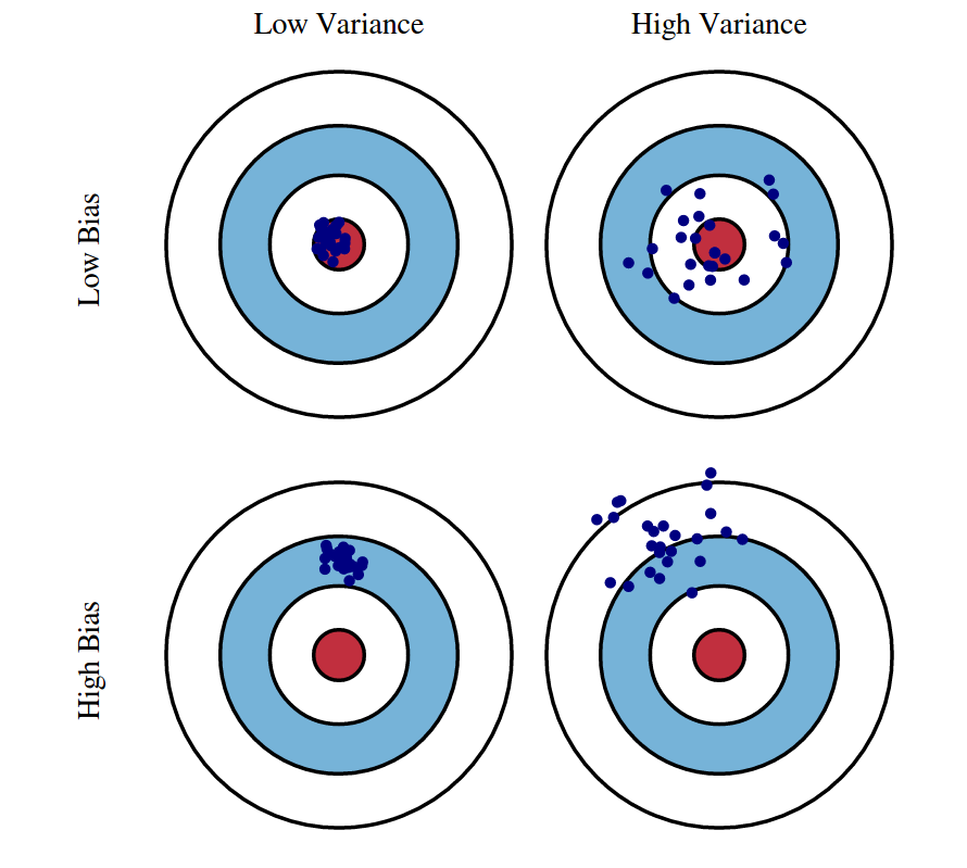
Fig 1: Graphical illustration of bias and variance.
Source: http://scott.fortmann-roe.com/docs/BiasVariance.html

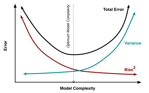
Fig 2: The variation of Bias and Variance with the model complexity. This is similar to the concept of overfitting and underfitting. More complex models overfit while the simplest models underfit.
Source: http://scott.fortmann-roe.com/docs/BiasVariance.html