10: Empirical Risk Minimization

Recap

Remember the Unconstrained SVM Formulation \[ \min_{\mathbf{w}}\ C\underset{Hinge-Loss}{\underbrace{\sum_{i=1}^{n}max[1-y_{i}\underset{h({\mathbf{x}_i})}{\underbrace{(w^{\top}{\mathbf{x}_i}+b)}},0]}}+\underset{l_{2}-Regularizer}{\underbrace{\left\Vert w\right\Vert _{z}^{2}}} \] The hinge loss is the SVM's loss/error function of choice, whereas the $\left.l_{2}\right.$-regularizer reflects the complexity of the solution, and penalizes complex solutions. Unfortunately, it is not always possible or practical to minimize the true error, since it is often not continuous and/or differentiable. However, for most Machine Learning algorithms, it is possible to minimize a "Surrogate" Loss Function, which can generally be characterized as follows: \[ \min_{\mathbf{w}}\frac{1}{n}\sum_{i=1}^{n}\underset{Loss}{\underbrace{l_{(s)}(h_{\mathbf{w}}({\mathbf{x}_i}),y_{i})}}+\underset{Regularizer}{\underbrace{\lambda r(w)}} \] ...where the Loss Function is a continuous function which penalizes training error, and the Regularizer is a continuous function which penalizes classifier complexity. Here we define $\lambda$ as $\frac{1}{C}$.^[1] The science behind finding an ideal loss function and regularizer is known as Empirical Risk Minimization or Structured Risk Minimization.

Commonly Used Binary Classification Loss Functions

Different Machine Learning algorithms employ their own loss functions; Table 4.1 shows just a few:

Loss $\ell(h_{\mathbf{w}}(\mathbf{x}_i,y_i))$	Usage	Comments
1.Hinge-Loss $max\left[1-h_{\mathbf{w}}(\mathbf{x}_{i})y_{i},0\right]^{p}$	Standard SVM($\left.p=1\right.$) (Differentiable) Squared Hingeless SVM ($\left.p=2\right.$)	When used for Standard SVM, the loss function denotes margin length between linear separator and its closest point in either class. Only differentiable everywhere at $\left.p=2\right.$.
2.Log-Loss $\left.log(1+e^{-h_{\mathbf{w}}(\mathbf{x}_{i})y_{i}})\right.$	Logistic Regression	One of the most popular loss functions in Machine Learning, since its outputs are very well-tuned.
3.Exponential Loss $\left. e^{-h_{\mathbf{w}}(\mathbf{x}_{i})y_{i}}\right.$	AdaBoost	This function is very aggressive. The loss of a mis-prediction increases exponentially with the value of $-h_{\mathbf{w}}(\mathbf{x}_i)y_i$.
4.Zero-One Loss $\left.\delta(\textrm{sign}(h_{\mathbf{w}}(\mathbf{x}_{i}))\neq y_{i})\right.$	Actual Classification Loss	Non-continuous and thus impractical to optimize.

Table 4.1: Loss Functions With Classification $\left.y\in\{-1,+1\}\right.$

Quiz: What do all these loss functions look like with respect to $\left.z=y*h({\vec x})\right.$?

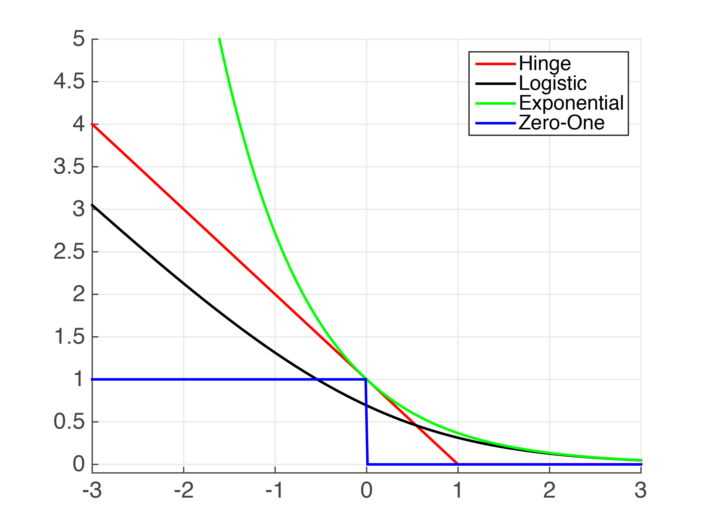
Figure 4.1: Plots of Common Classification Loss Functions - x-axis: $\left.h(\mathbf{x}_{i})y_{i}\right.$, or "correctness" of prediction; y-axis: loss value

Some additional notes on loss functions:

1. As hinge-loss decreases, so does training error.

2. As $\left.z\rightarrow-\infty\right.$, the log-loss and the hinge loss become increasingly parallel.

3. The exponential loss and the hinge loss are both upper bounds of the zero-one loss. (For the exponential loss, this is an important aspect in Adaboost, which we will cover later.)

4. Zero-one loss is zero when the prediction is correct, and one when incorrect.

Commonly Used Regression Loss Functions

Regression algorithms (where a prediction can lie anywhere on the real-number line) also have their own host of loss functions:

Loss $\ell(h_{\mathbf{w}}(\mathbf{x}_i,y_i))$						Comments
1.Squared Loss $\left.(h(\mathbf{x}_{i})-y_{i})^{2}\right.$						Most popular regression loss function Estimates Mean Label ADVANTAGE: Differentiable everywhere DISADVANTAGE: Somewhat sensitive to outliers/noise Also known as Ordinary Least Squares (OLS)
2.Absolute Loss $\left.\|h(\mathbf{x}_{i})-y_{i}\|\right.$						Also a very popular loss function Estimates Median Label ADVANTAGE: Less sensitive to noise DISADVANTAGE: Not differentiable at $0$
3.Huber Loss $\left.\frac{1}{2}\left(h(\mathbf{x}_{i})-y_{i}\right)^{2}\right.$ if $\|h(\mathbf{x}_{i})-y_{i}\|<\delta$, otherwise $\left.\delta(\|h(\mathbf{x}_{i})-y_{i}\|-\frac{\delta}{2})\right.$						Also known as Smooth Absolute Loss ADVANTAGE: "Best of Both Worlds" of Squared and Absolute Loss Once-differentiable Takes on behavior of Squared-Loss when loss is small, and Absolute Loss when loss is large.
4.Log-Cosh Loss $\left.log(cosh(h(\mathbf{x}_{i})-y_{i}))\right.$, $\left.cosh(x)=\frac{e^{x}+e^{-x}}{2}\right.$						ADVANTAGE: Similar to Huber Loss, but twice differentiable everywhere

Table 4.2: Loss Functions With Regression, i.e. $\left.y\in\mathbb{R}\right.$

Quiz: What do the loss functions in Table 4.2 look like with respect to $\left.z=(h(\mathbf{x}_{i})-y_{i})^{2}\right.$?

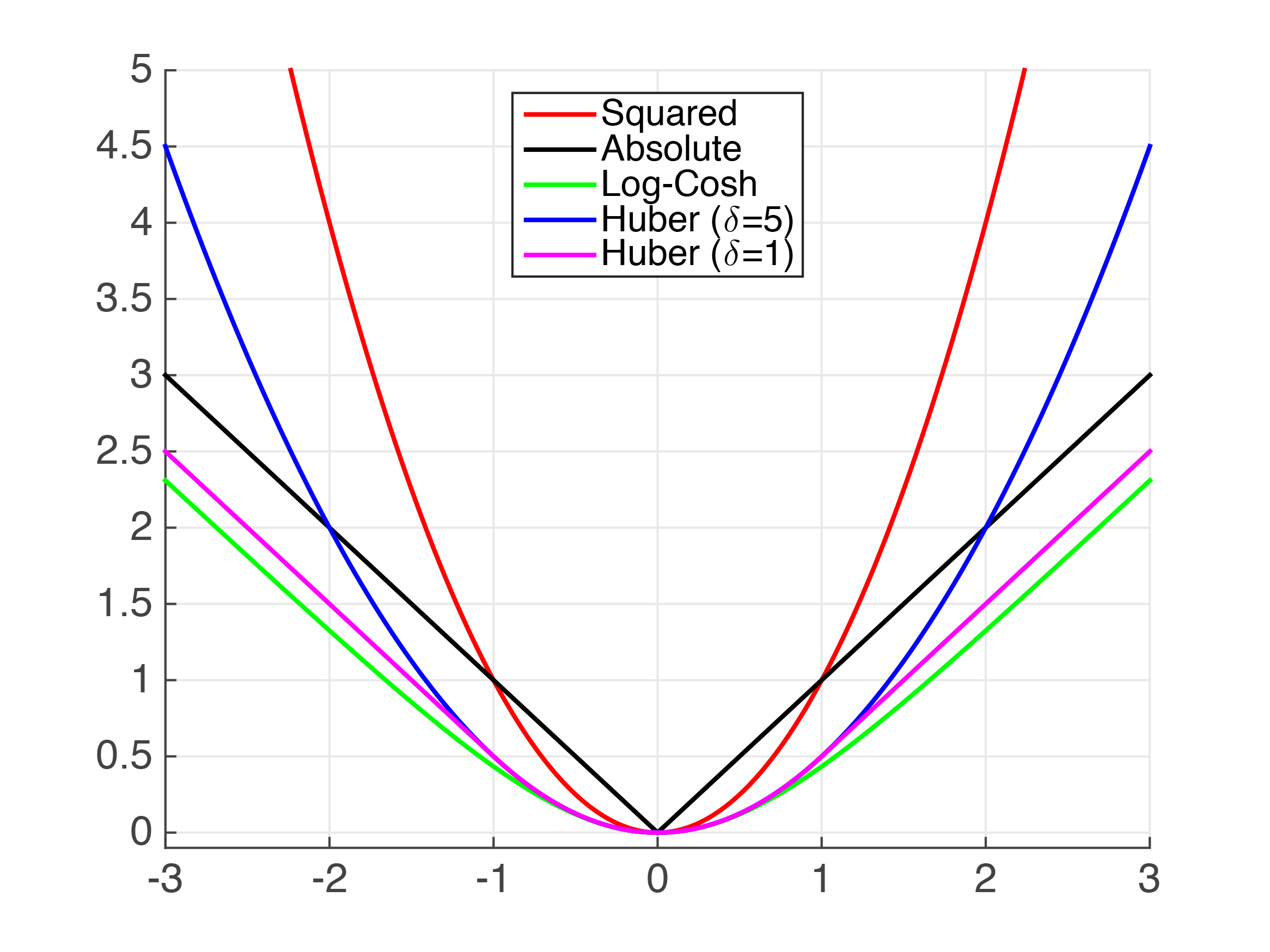
Figure 4.2: Plots of Common Regression Loss Functions - x-axis: $\left.h(\mathbf{x}_{i})y_{i}\right.$, or "error" of prediction; y-axis: loss value

Regularizers

\begin{equation} \min_{\mathbf{w},b} \sum_{i=1}^n\ell(\mathbf{w}^\top \vec x_i+b,y_i)+\lambda r(\mathbf{w}) \Leftrightarrow \min_{\mathbf{w},b} \sum_{i=1}^n\ell(\mathbf{w}^\top \vec x_i+b,y_i) \textrm { subject to: } r(w)\leq B \end{equation} For each $\left.\lambda\geq0\right.$, there exists $\left.B\geq0\right.$ such that the two formulations in (4.1) are equivalent, and vice versa. In previous sections, $\left.l_{2}\right.$-regularizer has been introduced as the component in SVM that reflects the complexity of solutions. Besides the $\left.l_{2}\right.$-regularizer, other types of useful regularizers and their properties are listed in Table 4.3.

Regularizer $r(\mathbf{w})$						Properties
1.$l_{2}$-Regularization $\left.r(\mathbf{w}) = \mathbf{w}^{\top}\mathbf{w} = (\\|{\mathbf{w}}\\|_{2})^{2}\right.$						ADVANTAGE: Strictly Convex ADVANTAGE: Differentiable DISADVANTAGE: Uses weights on all features, i.e. relies on all features to some degree (ideally we would like to avoid this) - these are known as Dense Solutions.
2.$l_{1}$-Regularization $\left.r(\mathbf{w}) = \\|\mathbf{w}\\|_{1}\right.$						Convex (but not strictly) DISADVANTAGE: Not differentiable at $0$ (the point which minimization is intended to bring us to Effect: Sparse (i.e. not Dense) Solutions
3.Elastic Net $\left.\alpha\\|\mathbf{w}\\|_{1}+(1-\alpha)(\\|{\mathbf{w}}\\|_{2})^{2}\right.$ $\left.\alpha\in[0, 1)\right.$						ADVANTAGE: Strictly convex (i.e. unique solution) DISADVANTAGE: Non-differentiable
4.lp-Norm often $\left.0<p\leq1\right.$ $\left.\\|{\mathbf{w}}\\|_{p} = (\sum\limits_{i=1}^d v_{i}^{p})^{1/p}\right.$						DISADVANTAGE: Non-convex ADVANTAGE: Very sparse solutions Initialization dependent DISADVANTAGE: Not differentiable

Table 4.3: Types of Regularizers

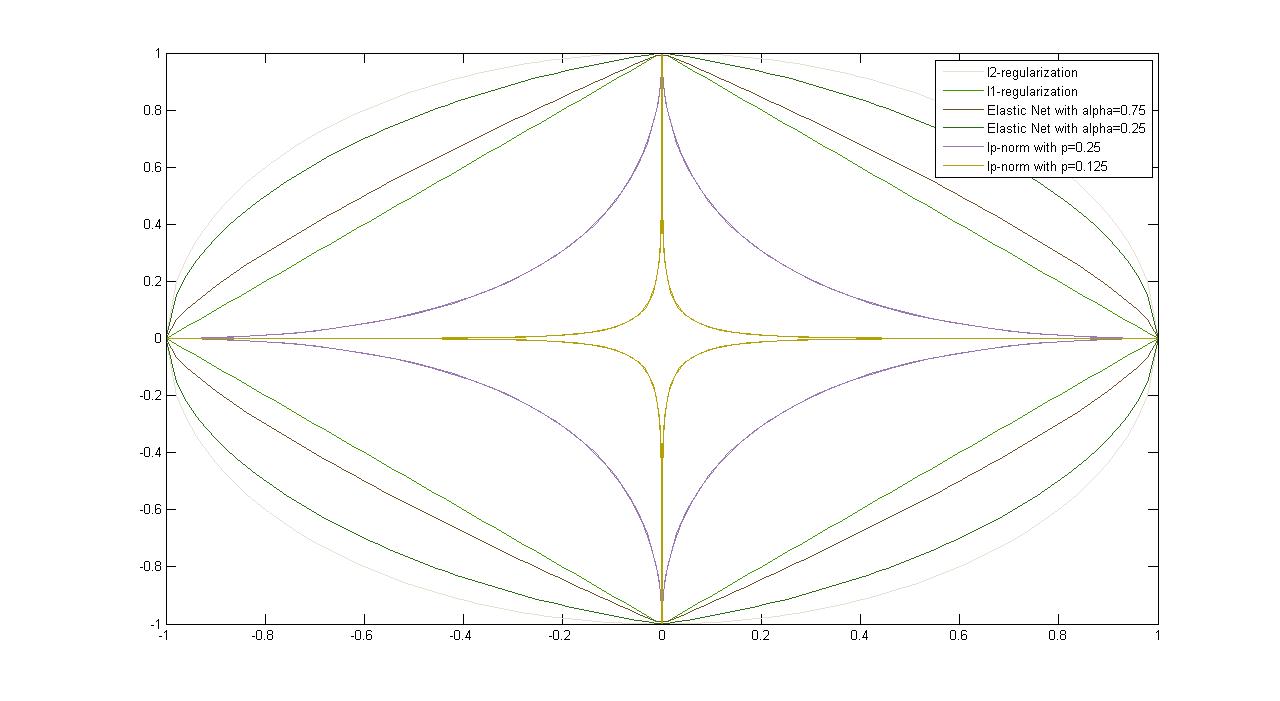
Figure 4.3: Plots of Common Regularizers

Famous Special Cases

This section includes several special cases that deal with risk minimization, such as Ordinary Least Squares, Ridge Regression, Lasso, and Logistic Regression. Table 4.4 provides information on their loss functions, regularizers, as well as solutions.

Loss and Regularizer	Classification	Solutions
1.Ordinary Least Squares $\min_{\mathbf{w}} \frac{1}{n}\sum\limits_{i=1}^n (\mathbf{w}^{\top}x_{i}-y_{i})^{2}$	Squared Loss No Regularization	$\left.\mathbf{w}=(\mathbf{X}\mathbf{X}^\top)^{-1}\mathbf{X}\mathbf{y}^{\top}\right.$ $\left.X=[\mathbf{x}_{1}, ..., \mathbf{x}_{n}]\right.$ $\left.Y=[y_{1},...,y_{n}]\right.$
2.Ridge Regression $\min_{\mathbf{w}} \frac{1}{n}\sum\limits_{i=1}^n (\mathbf{w}^{\top}x_{i}-y_{i})^{2}+\lambda\\|{w}\\|_{2}^{2}$	Squared Loss $l_{2}$-Regularization	$\left.w=(\mathbf{X}\mathbf{X}^{\top}+\lambda\mathbb{I})^{-1}\mathbf{X}^\top\mathbf{y}^{\top}\right.$
3.Lasso $\min_{\mathbf{w}} \frac{1}{n}\sum\limits_{i=1}^n (\mathbf{w}^{\top}\mathbf{x}_{i}-\vec{y_{i}})^{2}+\lambda\\|\mathbf{w}\\|_{1}$	+ sparsity inducing (good for feature selection) + Convex - Not strictly convex (no unique solution) - Not differentiable (at 0)	Solve with (sub)-gradient descent or SVEN
4.Logistic Regression $\min_{\mathbf{w},b} \frac{1}{n}\sum\limits_{i=1}^n \log{(1+e^{-y_i(\mathbf{w}^{\top}\mathbf{x}_{i}+b)})}$	Often $l_{1}$ or $l_{2}$ Regularized	Estimation: $\left.\Pr{(y=+1\|x)}=\frac{1}{1+e^{-y(\mathbf{w}^{\top}x+b)}}\right.$

Table 4.4: Special Cases

Some additional notes on the Special Cases:

1. Ridge Regression is very fast if data isn't too high dimensional.

2. Ridge Regression is one of the first ways to optimize in MATLAB in a Machine Learning setting.

3. A noteworthy counterpart to Ordinary Least Squares is PCA (Principal Component Analysis) also minimizes square loss, but looks at perpendicular loss (the horizontal distance between each point and the regression line) instead.

[1] In Bayesian Machine Learning, it is possible to optimize $\lambda$, but for the purposes of this class, it is assumed to be fixed.