Bayes Classifier and Naive Bayes
Idea: Estimate $\hat{P}(y | \vec{x})$ from the data, then use the Bayes Classifier on $\hat{P}(y|\vec{x})$.
So how can we estimate $\hat{P}(y | \vec{x})$?
One way to do this would be to use the MLE method. Assuming that $y$ is discrete,
$$
\hat{P}(y|\vec{x}) = \frac{\sum_{i=1}^{n} I(\vec{x}_i = \vec{x} \wedge \vec{y}_i = y)}{ \sum_{i=1}^{n} I(\vec{x}_i = \vec{x})}
$$
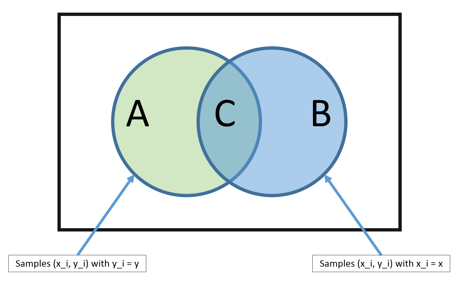 From the above diagram, it is clear that, using the MLE method, we can estimate $\hat{P}(y|\vec{x})$ as
$$
\hat{P}(y|\vec{x}) = \frac{|C|}{|B|}
$$
But there is a big problem with this method.
Problem: The MLE estimate is only good if there are many training vectors with the same identical features as
$\vec{x}$!
In high dimensional spaces (or with continuous $\vec{x}$), this never happens! So $|B| \rightarrow 0$ and $|C| \rightarrow 0$.
To get around this issue, we can make a 'naive' assumption.
From the above diagram, it is clear that, using the MLE method, we can estimate $\hat{P}(y|\vec{x})$ as
$$
\hat{P}(y|\vec{x}) = \frac{|C|}{|B|}
$$
But there is a big problem with this method.
Problem: The MLE estimate is only good if there are many training vectors with the same identical features as
$\vec{x}$!
In high dimensional spaces (or with continuous $\vec{x}$), this never happens! So $|B| \rightarrow 0$ and $|C| \rightarrow 0$.
To get around this issue, we can make a 'naive' assumption.
Naive Bayes
We can approach dilemma with a simple trick, and an additional assumption. The trick part is to estimate $P(y)$ and $P(\vec{x} | y)$ instead, since, by Bayes rule,
$$
P(y | \vec{x}) = \frac{P(\vec{x} | y)P(y)}{P(\vec{x})}
$$
Estimating $P(y)$ is easy. If $Y$ takes on discrete binary values, for example, this just becomes coin tossing. Also, recall from
Estimating Probabilities from Data
that estimating $P(y)$ and $P(\vec{x} | y)$ is called genreative learning.
Estimating $P(\vec{x}|y)$, however, is not easy! (you will explore this in the written homework).
The additional assumption that we make is the Naive Bayes assumption.
Naive Bayes Assumption:
$$
P(\vec{x} | y) = \prod_{\alpha = 1}^{d} P([\vec{x}]_\alpha | y)
$$
i.e. Feature values are independent given the label! This is a very bold assumption.
As a quick example, suppose that you want to predict the label that indicates if you have the flu or not ($Y \in \{\text{yes flu}, \text{no flu}\}$)
And you want to predict this using binary features on caughing, fever. Under the naive assumption, if I know that a person
has the flu, then knowing that the person is also caughing does not change the probability that the person has a fever.
It is clear that this is not the case in reality.
But, for now, let's assume that it holds.
Then the Bayes Classifier can be defined as
\begin{align}
h(\vec{x}) &= argmax_y P(y | \vec{x}) \\
&= argmax_y \frac{P(\vec{x} | y)P(y)}{P(\vec{x})} \\
&= argmax_y P(\vec{x} | y) P(y) && \text{($P(\vec{x})$ does not depend on $y$)} \\
&= argmax_y \prod_{\alpha=1}^{d} P([\vec{x}]_\alpha | y) P(y) && \text{(By the naive assumption)}\\
&= argmax_y \sum_{\alpha = 1}^{d} log(P([\vec{x}]_\alpha | y)) + log(P(y)) && \text{(As log is a monotonic function)}
\end{align}
Estimating $log(P([\vec{x}]_\alpha | y))$ is easy as we only need to consider one dimension. And estimating $P(y)$
is not affected by the assumption, but it is still easy.
Estimating $P([\vec{x}]_\alpha | y)$
Now that we know how we can use our assumption to make estimation of $P(y|\vec{x})$ tractable,
let's move on and look at how we can actually apply our method to different problems.
There are 3 notable cases in which we can use our naive Bayes classifier.
Case #1: Categorical features
Features:
$$[\vec{x}]_\alpha \in \{f_1, f_2, \cdots, f_{K_\alpha}\}$$
Each feature $\alpha$ falls into one of $K_\alpha$ categories.
(Note that the case with binary features is just a specific case of this)
Model:
$$
P([\vec{x}]_{\alpha} = j | y) = [p_{j}^{y}]_{\alpha} \\
\text{ where } \sum_{j=1}^{k} [p_{j}^{y}]_{\alpha} = 1
$$
where $[p_{j}^{y}]_{\alpha} $ is the probability of feature $\alpha$ having the value $j$, given that the label is $y$.
And the constraint indicates that $[\vec{x}]_{\alpha}$ must have one of $\{1, \cdots, k\}$.
Estimator:
\begin{align}
[p_{j}^{y}]_{\alpha} &= \frac{\sum_{i=1}^{n} I(y_i = y \wedge [\vec{x}_i]_\alpha = j) + l}{\sum_{i=1}^{n} I(y_i = y) + lk}
\end{align}
where $l$ is the smoothing constant.
Case #2: Multinomial features
Features:
\begin{align}
[\vec{x}]_\alpha \in \{0, 1, 2, \cdots \} && \text{(Each feature $\alpha$ represents a count)}
\end{align}
An example of this could be the count of a specific word $\alpha$ in a document.
Model:
\begin{align}
P([\vec{x}]_1 = j_1,\dots,[\vec{x}]_d = j_d | y) = \frac{m!}{j_1!\dots j_d!}([p^{y}]_{1})^{j_1}\dots ([p^{y}]_{d})^{j_d} && \text{and} && \sum_{\alpha = 1}^{d} [p^y]_\alpha = 1 && \textrm{where $m=\sum_{\alpha=1}^n j_\alpha$}
\end{align}
So, for example, if there are $d$ number of words in the vocabulary, each word $\alpha$ has some probability mass
of being spam of ham. For both cases, $y = \text{spam}$ and $y = \text{ham}$, the probabilities sum to 1.
Estimator:
\begin{align}
[p^y]_\alpha = \frac{\sum_{i = 1}^{n} I(y_i = y)[\vec{x}]_\alpha + l}{\sum_{i=1}^{n}\sum_{\beta = 1}^{d} [\vec{x}]_{\beta} I(y_i = y) + dl }
\end{align}
Case #3: Continuous features (Gaussian Naive Bayes)
Features:
\begin{align}
[\vec{x}]_\alpha \in \mathbb{R} && \text{(each feature takes on a real value)}
\end{align}
Model:
\begin{align}
P([\vec{x}]_\alpha | y) = \mathcal{N}([\vec{\mu}_y]_\alpha, [\vec{\sigma}_{y}^{2}]_\alpha)
\end{align}
Note that the model specified above is based on our assumption about the data - that each feature $\alpha$ comes from a class-conditional Gaussian distribution.
Other specification could be used as well.
Estimator:
\begin{align}
[\vec{\mu}_y]_\alpha &\leftarrow \frac{1}{n_y} \sum_{i = 1}^{n} I(y_i = y) [\vec{x}]_\alpha && \text{where $n_y = \sum_{i=1}^{n} I(y_i = y)$} \\
[\vec{\sigma}_y^2]_\alpha &\leftarrow \frac{1}{n_y} \sum_{i=1}^{n} I(y_i = y)([\vec{x}_i]_\alpha - [\vec{\mu}_y]_\alpha)^2
\end{align}
Naive Bayes is a linear classifier
Suppose that $y_i \in \{-1, +1\}$ and features are multinomial ($P([\vec{x}]_\alpha | y) = $)
Let us define:
\begin{align}
[\vec{w}]_\alpha &= log(p_{\alpha}^{+1}) - log(p_{\alpha}^{-1}) \\
b &= log(P(Y = +1)) - log(P(Y = -1))
\end{align}
If we use the above to do classification, we can compute for $\vec{w}^T \cdot \vec{x} + b$
Simplifying this further leads to
\begin{align}
\vec{w}^T \cdot \vec{x} + b > 0 &\Longleftrightarrow \sum_{\alpha = 1}^{d} [\vec{x}]_\alpha (log(p_{\alpha}^{+1}) - log(p_{\alpha}^{-1})) + log(P(Y = +1)) - log(P(Y = -1)) > 0 \\
&\Longleftrightarrow \frac{\prod_{\alpha = 1}^{d} P([\vec{x}]_\alpha | Y = +1)P( Y = +1)}{\prod_{\alpha =1}^{d}P([\vec{x}]_\alpha | Y = -1)P(Y = -1))} > 0 \\
&\Longleftrightarrow P(Y = +1 | \vec{x}) > P(Y = -1 | \vec{x}) && \text{(By our naive Bayes assumption)} \\
&\Longleftrightarrow h(\vec{x}) = +1 && \text{(By definition of $h(\vec{x})$)}
\end{align}
Some extra notes related to lecture on 9/21/2015
I think there is some confusion about Naive Bayes with the multinomial distribution.
Let me explain it one more time in a different way.
The multinomial view:
Let us assume we have d possible words in our dictionary. We have a data instance (e.g. an email) consisting of m words.
Each of the $d$ words has a probability for spam
$p_1,\dots,p_d$ and for ham $q_1,\dots,q_d$ (with $\sum_{\alpha=1}^d p_\alpha=1=\sum_{\alpha=1}^d q_\alpha$.)
We also have probabilities that an email is spam $\pi_s$ and that it is ham $\pi_h$ with $\pi_s+\pi_h=1$.
If you want to generate an email, you follow the following procedure. First you decide with probability $\pi_s$ if you want to write a spam email or a ham email. Then you pick the corresponding probability distribution and randomly pick $m$ words.
$w_1,\dots,w_m$.
Each of these words is picked independently. So if you generate a spam email, the probability that the first term is word $\alpha$ is $p_\alpha$.
Let us write $w_i=\alpha$ to denote that the $i^{th}$ word in the email was word $\alpha$, where $\alpha\in\{1,\dots,d\}$.
What is the probability that a particular email was generated that way, with the spam label (so we used $p_\alpha$ instead of $q_\alpha$)?
Keep in mind that in the bag of words representation word order does not matter and we are therefore mostly concerned with how many times each word appeared. Let these counts be $n_1,\dots, n_d$ to denote the occurrences of word 1, word 2, ... word d respectively (with $\sum_{\alpha=1}^d n_\alpha=m$).
To represent your email as a vector, you write $\vec x=[n_1,\dots,n_d]^\top$.
The multinomial distribution then specifies that the likelihood of the email is
\begin{align}
P(\vec x | Y=spam)=\frac{m!}{n_1!\times \dots \times n_d!}p_1^{n_1}\times \dots \times p_d^{n_d}
\end{align}
We don't actually need the exact likelihood, as we can decide the label by evaluating $\frac{P(Y=spam|\vec x)}{P(Y=ham|\vec x)}$. (If this fraction is greater than one the email is classified as spam otherwise ham.) In this fraction all normalization constants disappear as they are the same for spam and ham.
It is therefore enough to evaluate
$$
P(\vec x | Y=spam)\propto p_1^{n_1}\times \dots \times p_d^{n_d}
$$
This is exactly what we used in class.
You notice, that $m$ disappeared. So, to use naive bayes on document data we do not have to make any assumptions about the length of the document. We simply check if this particular document, no matter what its length is, contains words that are more likely to be generated with the spam generating process or with the ham generating process.
So the ratio we finally compute is:
\begin{align}
\frac{P(Y=spam| \vec{x})}{P(Y=ham|\vec x)}=\frac{P(\vec x|Y=spam)P(Y=spam)}{P(\vec x|Y=ham)P(Y=ham)}=\frac{p_1^{n_1}\times\dots\times p_d^{n_d}\times\pi_s}{q_1^{n_1}\times\dots\times q_d^{n_d}\times\pi_h}
\end{align}
How do we get the probabilities $p_\alpha$?
Well, $p_\alpha$ is the probability that word $\alpha$ is chosen to generate a spam email. So we can estimate it as the fraction of words in spam emails that are word $\alpha$:
$$p_\alpha=\frac{\textrm{no. of times word $\alpha$ appears in spam emails in our training data}}{\textrm{no. of words in all spam emails in our training data}}$$
-Kilian