CS4670/5670: Computer Vision, Spring 2015
Project 2:  Feature Detection and Matching

Brief

• Assigned:  Monday, February 23, 2015
• Code Due: Monday, March 9, 2015 (by 11:59pm) (turnin via CMS)
• Webpage Due: Tuesday, March 10, 2015 (by 11:59pm) (turnin via CMS)
• Teams:  This assignment must be done in groups of 2 students.

Synopsis

In this project, you will write code to detect discriminating features in an image and find the best matching features in other images.  Your features should be reasonably invariant to translation, rotation, and illumination. You will evaluate their performance on a suite of benchmark images. Watch this video to see the solution in action. You can also look at the slides presented in class.

In Project 3, you will apply your features to automatically stitch images into a panorama. 

To help you visualize the results and debug your program, we provide a user interface that displays detected features and best matches in other images.  We also provide an example ORB feature detector, a current best of breed technique in the vision community, for comparison.

Finally, to make programming easier, this assignment will be in Python, with the help of NumPy and SciPy. Python+NumPy+SciPy is a very powerful scientific computing environment, and makes computer vision tasks much easier. A crash-course on Python and NumPy can be found here.

Description

The project has three parts:  feature detection, feature description, and feature matching.

1. Feature detection

In this step, you will identify points of interest in the image using the Harris corner detection method.  The steps are as follows (see the lecture slides/readings for more details)  For each point in the image, consider a window of pixels around that point.  Compute the Harris matrix H for (the window around) that point, defined as

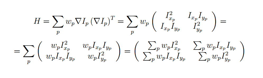
where the summation is over all pixels p in the window.  is the x derivative of the image at point p, the notation is similar for the y derivative. You should use the Sobel operator to compute the x, y derivatives. The weights should be chosen to be circularly symmetric (for rotation invariance).  You should use a 5x5 Gaussian mask with 0.5 sigma.

Note that H is a 2x2 matrix.  To find interest points, first compute the corner strength function

Once you've computed c for every point in the image, choose points where c is above a threshold.  You also want c to be a local maximum in a 7x7 neighborhood. In addition to computing the feature locations, you'll need to compute a canonical orientation for each feature, and then store this orientation (in degrees) in each feature element. To compute the canonical orientation at each pixel, you should compute the gradient (using the Sobel operator again) of the blurred image (with a Gaussian kernel with 7x7 window and 0.75 sigma) and use the angle of the gradient as orientation.

2. Feature description

Now that you've identified points of interest, the next step is to come up with a descriptor for the feature centered at each interest point.  This descriptor will be the representation you'll use to compare features in different images to see if they match.

You will implement two descriptors for this project. For starters, you will implement a simple descriptor, a 5x5 square window without orientation. This should be very easy to implement and should work well when the images you're comparing are related by a translation. Second, you'll implement a simplified version of the MOPS descriptor. You'll compute an 8x8 oriented patch sub-sampled from a 40x40 pixel region around the feature. You have to come up with a transformation matrix which transforms the 40x40 rotated window around the feature to the 8x8 patch, with a canonical orientation where 0 degree corresponds to the (1, 0) direction vector, i.e. the vector points to the right. You should also normalize the patch to have zero mean and unit variance.

3. Feature matching

Now that you've detected and described your features, the next step is to write code to match them, i.e., given a feature in one image, find the best matching feature in one or more other images.  This part of the feature detection and matching component is mainly designed to help you test out your feature descriptor.  You will implement a more sophisticated feature matching mechanism in the second component when you do the actual image alignment for the panorama.

The simplest approach is the following:  write a procedure that compares two features and outputs a distance between them.  For example, you could simply sum the absolute value of differences between the descriptor elements. You could then use this distance to compute the best match between a feature in one image and the set of features in another image by finding the one with the smallest distance. Two possible distances are:

1. The SSD (Sum of Squared Distances) distance. The SSD is implemented for you in class SSDFeatureMatcher. This basically means computing the Euclidean distance between the two feature vectors. You must implement this distance.
2. The Ratio test. Compute (SSD distance of the best feature match)/(SSD distance of the second best feature match) and store this value as the distance between the two feature vectors. This is called the "ratio test". You must implement this distance.

Testing

Now you're ready to go!  Using the UI and skeleton code that we provide, you can load in a set of images, view the detected features, and visualize the feature matches that your algorithm computes.

By running featuresUI.py, you will see a GUI where you have the following choices:

• Keypoint Detection
  You can load an image and compute the points of interest with their orientation.
• Feature Matching
  Here you can load two images and view the computed best matches using the specified algorithms.
• Benchmark
  After specifying the path for the directory containing the dataset, the program will run the specified algorithms on all images and compute ROC curves for each image.

You may use the UI to perform individual queries to see if things are working right. First you need to load a query image check if the detected key points have reasonable number and orientation under the Keypoint Detection tab. Then, you can check if your feature descriptors and matching algorithms work using the Feature Matching tab.

We are providing a set of benchmark images to be used to test the performance of your algorithm as a function of different types of controlled variation (i.e., rotation, scale, illumination, perspective, blurring).  For each of these images, we know the correct transformation and can therefore measure the accuracy of each of your feature matches.  This is done using a routine that we supply in the skeleton code.

You should also go out and take some photos of your own to see how well your approach works on more interesting data sets.  For example, you could take images of a few different objects (e.g., books, offices, buildings, etc.) and see if it can "recognize" new images.

Downloads

Virtual machine: We provide you with a VirtualBox virtual machine running Ubuntu with most of the necessary dependencies installed (password is 'student'). To install the remaining dependencies, run the following script on the machine:
Skeleton code: Available through git (this should help make distributing any updates easier). With git installed, you can download the code by typing (using the command-line interface to git) This will create the directory skeleton. To get updates to the code you can then simply run This will fetch any updates and merge them into your local copy. If we modify a file you have already modified git will not overwrite your changes. Instead, it will mark the file as having a conflict and then ask you to resolve how to integrate the changes from these two sources. Here's a quick guide on how to resolve these conflicts.

For those that are already using git to work in groups, you can still share code with your partner by having multiple masters to your local repository (one being this original repository and the other some remote service like github where you host the code you are working on); here's a reference with more information.

This skeleton code should run on the provided VM, without any further installation. We provide an installation script if you want to run it on a different machine. Download some image sets for benchmark: datasets.

To Do

We have given you a number of classes and methods to help get you started. We strongly advise you to read the documentation above the functions, which will help you understand the inputs and outputs of the functions you have to implement. The code you need to write will be for your feature detection methods, your feature descriptor methods and your feature matching methods, all in features.py. The feature computation and matching methods are called from the GUI functions in featuresUI.py.

1. We have provided a class DummyKeypointDetector that shows how to create basic code for detecting features, and integrating them into the rest of the system. Here you can see which fields of the cv2.KeyPoint you should fill in. In the assignment we use the size attribute only for visualization, you should set it to 10. You should set the pt (coordinate), size, response (key point detector response, for the Harris detector, this is the Harris score at the pixel) and angle (in degrees) attributes for each keypoint.
2. The function detectKeypoints in HarrisKeypointDetector is one of the main ones you will complete, along with the helper functions computeHarrisValues (computes Harris scores and orientation for each pixel in the image) and computeLocalMaxima (computes a binary array which tells for each pixel if it is a local maximum). These implement Harris corner detection. For filtering the image and computing the gradients, you can either use the following functions or implement you own filtering code as you did in the first assignment:
   • scipy.ndimage.sobel: Filters the input image with Sobel filter.
   • scipy.ndimage.gaussian_filter: Filters the input image with a Gaussian filter.
   • scipy.ndimage.filters.maximum_filter: Filters the input image with a maximum filter.
   • scipy.ndimage.filters.convolve: Filters the input image with the selected filter.
   • You are also free to use numpy functions and numpy array arithmetic for efficient and concise implementation.
   You can look up these functions here. When using the Sobel operator, you should use the default settings for padding (i.e. you don't have to specify anything for padding). The default setting is 'reflect', which gives 0 gradient at the edges.
3. You'll need to implement two feature descriptors in SimpleFeatureDescriptor and MOPSFeaturesDescriptor classes. The describeFeatures function of these classes take the location and orientation information already stored in a set of key points (e.g., Harris corners), and compute descriptors for these key points, then store these descriptors in a numpy array which has the same number of rows as the computed key points and columns as the dimension of the feature (5x5 = 25 for SimpleFeatureDescriptor).
   For the MOPS implementation, you can use the transformation matrix helper functions defined in transformations.py. You have to create a matrix, which transforms the 40x40 patch around the key point to canonical orientation and scales it down by 5, as described on the lectures slides. For further details about how cv2.warpAffine works, please look at the opencv documentation.
4. Finally, you'll implement a function for matching features. You will implement the matchFeatures function of SSDFeatureMatcher and RatioFeatureMatcher. To efficiently compute the distances between all feature pairs between the two images, you can use scipy.spatial.distance.cdist. To determine the best match, you can use numpy functions such as argmin, but you can implement everything by yourself if you prefer.
   These functions should return a list of cv2.DMatch objects. You should set the queryIdx attribute to the index of the feature in the first image, the trainIdx attribute to the index of the feature in the second image and the distance attribute to the distance between the two features as defined by the particular distance metric (e.g., SSD or ratio).
5. You will also need to generate plots of the ROC curves and report the areas under the ROC curves (AUC) for your feature detecting and matching code and for ORB. For both the Yosemite dataset and the graf dataset, create 6 plots with the GUI, two using the simple window descriptor and simplified MOPS descriptor with the SSD distance, two using these two types of descriptors with the ratio test distance, and the other two using ORB (with both the SSD and ratio test distances). You can create these plots on the Benchmark tab.
6. Finally, you will need to report the average AUC for your feature detecting and matching code (using the Benchmark tab on the GUI again) on four benchmark sets: graf, leuven, bikes and wall.

Here is a summary of potentially useful functions (you do not have to use any of these):

• scipy.ndimage.sobel
• scipy.ndimage.gaussian_filter
• scipy.ndimage.filters.convolve
• scipy.ndimage.filters.maximum_filter
• scipy.spatial.distance.cdist
• cv2.warpAffine
• np.max, np.min, np.std, np.mean, np.argmin, np.argpartition
• np.degrees, np.radians, np.arctan2
• transformations.get_rot_mx (in transformations.py)
• transformations.get_trans_mx
• transformations.get_scale_mx

What to Turn In

First, your source code and executable should be zipped up into an archive called 'code.zip', and uploaded to CMS. In addition, turn in a web page describing your approach and results (in an archive called 'webpage.zip').  In particular:

• Explain why you made the major design choices that you did
• Report the performance (i.e., the ROC curve and AUC) on the provided benchmark image sets
1. You will need to compute two sets of 6 ROC plots and post them on your web page as described in the above TO DO section. You can learn more about ROC curves from the class slides and on the web here and here.
2. For one image each in both the Yosemite and graf test pairs, please include an image of the Harris operator on your webpage.  This image can be saved clicking on the Screenshot button under the Keypoint Detection tab.
3. Report the average AUC for your feature detecting (simple 5x5 window descriptor, MOPS descriptor and your own new descriptor) and matching code (both SSD and ratio tests) on four benchmark sets graf, leuven, bikes and wall.
• Describe strengths and weaknesses
• Take some images yourself and show the performance (include some pictures on your web page!)
• Describe any extra credit items that you did (if applicable)

We will tabulate the best performing features and present them to the class.

The web-page (.html file) and all associated files (e.g., images, in JPG format) should be placed in a zip archive called 'webpage.zip' and uploaded to CMS. If you are unfamiliar with HTML you can use any web-page editor such as FrontPage, Word, or Visual Studio 7.0 to make your web-page.

Extra Credit

Here is a list of suggestions for extending the program for extra credit. You are encouraged to come up with your own extensions as well!

• Design and implement your own feature descriptor.
• Implement adaptive non-maximum suppression (MOPS paper)
• Make your feature detector scale invariant.
• Implement a method that outperforms the above ratio test for deciding if a feature is a valid match.
• Use a fast search algorithm to speed up the matching process.  You can use code from the web or write your own (with extra credit proportional to effort).  Some possibilities in rough order of difficulty:  k-d trees (code available here), wavelet indexing (see the MOPS paper), locality-sensitive hashing.

Acknowledgements

The instructor is extremely thankful to Prof. Steve Seitz for allowing us to use their project as a base for our assignment.

 

Last modified on February 21, 2015