Introduction

Our goal for this project is to create an augmented reality application for the Nokia N900. The application will take in a video stream from the camera and draw additional objects into the scene. In order to do so, however, we must know where the camera is and which way it is pointed relative to the objects in the 3D scene. Thus, we must first calculate the camera’s pose and then calculate a projection which we can use to project virtual objects into the scene.

The general problem of finding camera pose is complicated by the fact that we don’t know where objects in the image actually are in the scene. This is the general structure from motion problem, and is computationally intensive. In order to do pose tracking in real time, we use a fast-to-detect planar marker in the scene that we can define as a known location in the scene. By comparing the marker features in the image against these known locations, we can figure out where the camera is relative to it. Once we have done so, we can then render additional objects into the 3D scene by calculating which points they will project to in the image.

Related work

The problem of camera pose estimation has been widely tackled, and several algorithms have been developed to solve this problem. These algorithms fall into two groups: analytical and iterative (1, 6, 7). Analytical algorithms attempt to solve the problem via a closed solution, usually with some simplifying model assumptions (2, 5). Iterative algorithms use some error metric, usually based on some kind of projection compared with their actual measured correspondences. Iterative algorithms tend to be more widely used, because their results are usually accurate, and they take only a few iterations when seeded with a good initial guess (1, 3, 6, 7, 8, 10). To generate these guesses, some iterative algorithms take advantage of the derived analytical closed-form equations. Solving this pose estimation problem involves finding R and T, the rotation matrix and the translation vector that describe the camera position and orientation in the world coordinate systems. Error metrics therefore come usually in two flavors. The first is the sum of the squared errors between measured pixel points and the projections of the 3d world points that those pixel points correspond to. The second involves summing the squared errors between actual 3d world points and world points implied by the measured pixel point locations (3).

A minimum of 4 non-collinear point correspondences between the image and world is required to solve this problem exactly. This equivalently translates into 3 line correspondences, and algorithms have been designed which fore-go points for lines (9, 10). One of the simpler methods for generating these points is to find and use an object of known structure in the scene. But marker-less algorithms have been explored (8).

Framework

The Qt framework was used along with OpenCV to implement the phone application. The video stream was opened using OpenCV, which provides a simple interface for grabbing successive frames. This was used in favor of FCam for low resolution images. Because there was no way to control the exposure setting in the OpenCV video capture process, we needed to implement a color threshold method that was more invariant to illumination conditions.

Marker Detection

Camera pose calculation from one frame to the other requires information about objects that are viewable in the frames. Information can usually be obtained from the images by calculating the features of the objects using a feature extraction method such as SIFT or SURF. These features have to be unique for a particular object so that we can efficiently track them between frames, otherwise we might experience ambiguity if multiple features of a similar kind are present. Therefore, we decided to use unique circular color markers for our images such that they are easy to detect.

The next issue we faced was speed. Since the application had to be run on the Nokia N900 phone, we could not use methods such as SIFT or SURF because they required a lot of time to compute features in the images and match them between frames. Thus, decided to use a thresholding technique to detect the location of colored markers in the frame. The following paragraphs explain how this method was implemented.

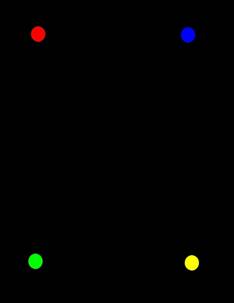
Figure: Marker Image used for tracking pose of camera

The 4 markers, as indicated by the above image were colored as high intensity values in the RGB channels (Yellow is high in Red and Green). These markers would have the most variation in the in each of the RGB channels as compared to its surrounding black image. Thus, a set of 15-20 images were taken in different illuminations and the minimum variation between the RGB channels was calculated to estimate the threshold of the markers. These thresholds were thus for relative change in channel intensity. To take an example, consider the red marker. The intensity of the red channel at the marker was calculated and compared against the blue and green channel to calculate variation. This variation was compared with a threshold to distinguish whether a pixel belonged to a particular marker. This method would be somewhat invariant to the illumination of the marker as well because we compare the relative change in channel intensities.

Using the threshold values calculated by the method above, each of the RGB channels were compared to form a binary channels channel for the RGB colors and a separate binary channel for the yellow marker. Thus, a transition from the black background to a particular marker would be a transition from 0 to 1 in their respective channels (which is very fast and easy to detect). The following method was used to detect the center of marker visible in the image.

Figure: Marker image from camera with green scan line drawn (left), Zoomed view of green marker with center estimation (top right), Zoomed view of green marker in the green binary image with center estimation (bottom right)

Figure: Original marker image and binary channels created using thresholding

The above image gives an illustration of the method used to find the center of a particular marker in the image. The entire area of the image was scanned from top to bottom and for every row, each channel was evaluated for find the start of marker transition (0 to 1) and its end (1 to 0). For a unique marker, we checked the marker constraints against the 3 channels validate the type of marker detected. Thus for a green marker, the green binary channel should give a 1 and red and blue should give a 0 (and so on). Thus for every scan line, the highest number of marker pixels found in a given row was stored. If a new row gave a larger count, the marker count and the row number would be updated. Thus the largest row calculated for each marker type was considered as the equator of the marker (this is basically the green dotted line that is contained within the marker in the above image). The center of this line was taken to be the center of the marker. This gave very accurate results for the marker positions from frame to frame and thus, resulted in good pose estimation. Extensive research was conducted to find a fast marker detector but most of the methods used some form of filtering using a kernel to find a particular feature in the environment. This would have proved to be more time consuming than the current method as it would have required convolution with several kernels (9 multiplications for every pixel and doing 4 of these for each of the marker), which is a lot more computation than the current implementation.

Augmentation

Once the system has identified the marker in terms of pixel locations of the 4 marker dots, it calls the function addShape, passing these as arguments. The addShape function constructs two matrices: a 4x4 matrix for the world points and a 3x4 matrix for the image points (both are in homogeneous form). Each column of these matrices is a point; the ith column of the image-points matrix corresponds to the measured projection of the world point i. The origin of the world coordinate system is the yellow dot on the marker, with the x direction along the yellow-blue line and the y direction along the yellow-green line. The z direction is upward perpendicular to the marker. The four world points are specified by dimensions W and H, which were measured to be 202 and 140 mm respectively.

Once the object-points and image-points matrices are created, the intrinsic matrix K is constructed using the focal length of the camera (5.2 mm) and the principle point, which is half the width and length of the image. In K, the focal length of the camera is converted into pixels at a rate of 84.6 px/mm. The function then uses cvFindExtrinsicCameraParams2 and cvRodrigues2 to generate the rotation matrix R and translation vector t. cvFindExtrinsicCameraParams2 uses an iterative algorithm minimizing the sum of squared errors between projected and actual image points to generate R and t. It assumes a projection matrix K[R|t]. Refer to the ‘related work’ section for a brief overview of some of the algorithms reviewed during this project.

Once R and t are known, the function creates the projection matrix. This can be used to project visible world point into the image. As a demonstration, we projected the four original marker points, along with four points at W/4 above them.

Results and Discussion

The final application runs between 1 and 2 frames per second on the phone, including saving a copy of the video to file. While this is not ideal, further speedups could be obtained with optimization. The main tradeoff came between implementing a more robust marker detector versus a faster marker detector. When using a simple threshold and centroid filter, the frame rate was around 5-7 fps. However, this method was not robust and as it would give large variations in the marker positions between frames. This was changed to implement the marker detector as explained in the above sections.

When the markers were found correctly, the results of the projection were of good quality and consistent between frames. This suggests that the error margins are fairly small for areas near the marker. We did not manage to test the code with the marker in a smaller portion of the scene, as the low resolution captures effectively limited how far away we could see the marker features from.

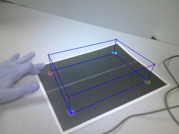
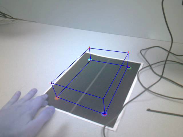
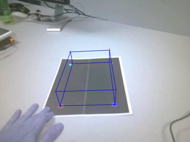
As a rudimentary proof of concept, we used the calculated extrinsics to draw a cube rising from the marker’s position.

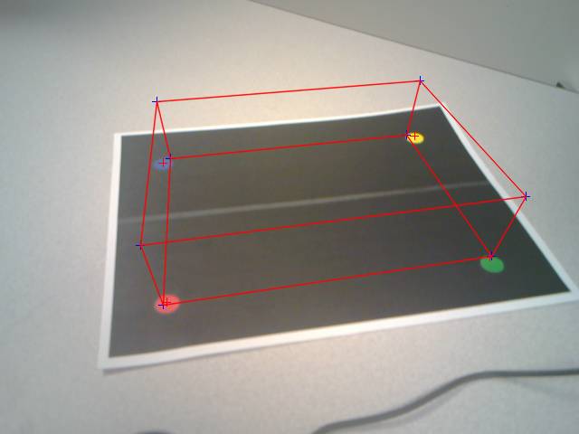
Figure: Cube drawn using estimated pose

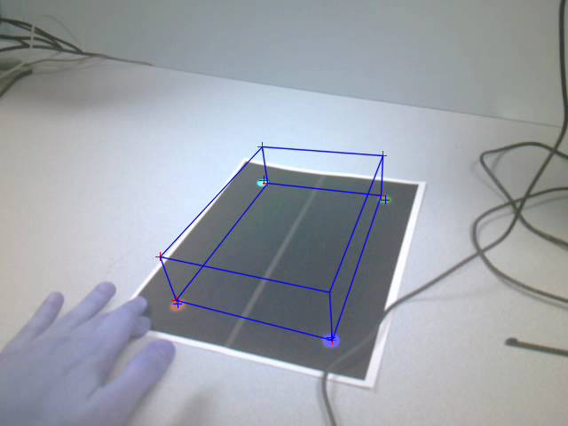
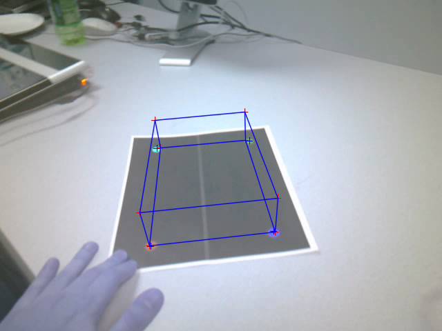
The points estimated in the above image were stable as the viewpoint of the camera moved around. The following images give the same cube from 2 different view angles (these were taken as snapshots from the saved video which had the R and B color channels reversed and thus, marker colors and cube drawn appear different). The blue and red channels were not flipped to RGB for video write in order to preserve video writing speed. The hand in the scene is not in fact frostbitten.

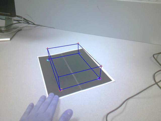
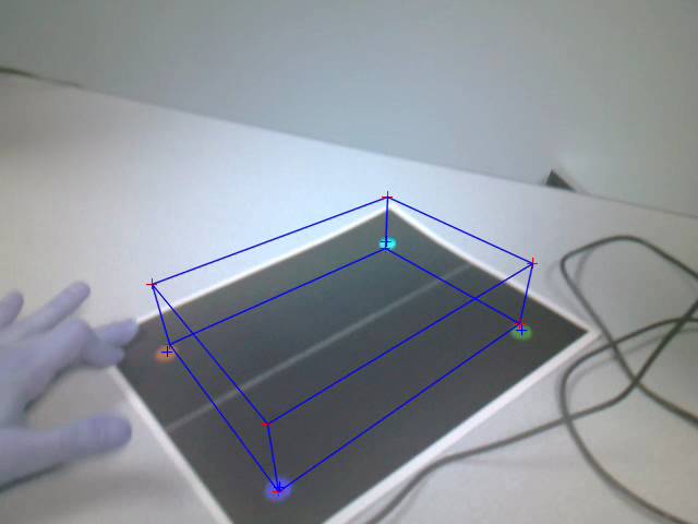
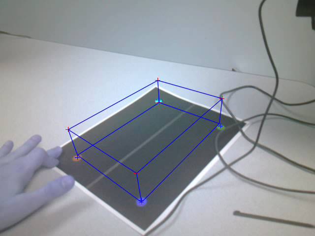
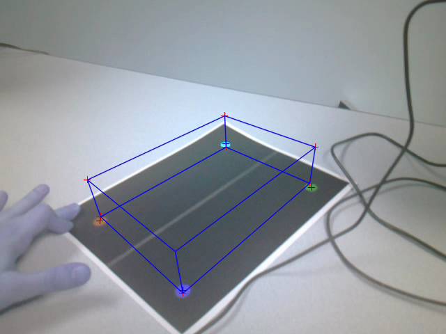
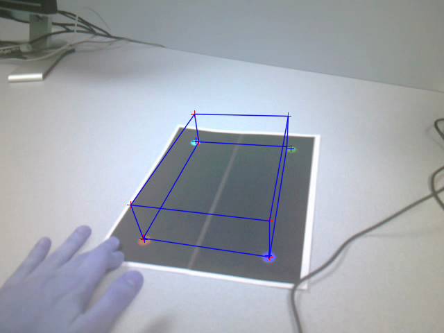
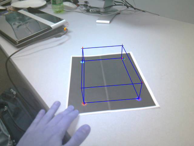
Figure: Cube drawn using estimated pose after movement

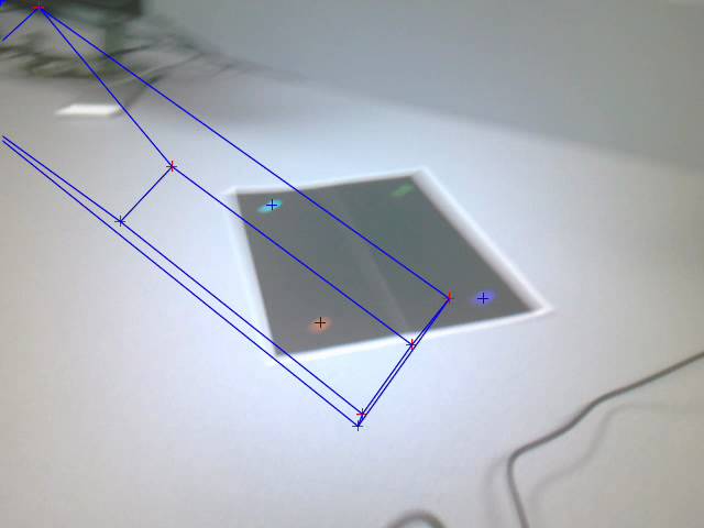
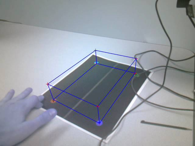
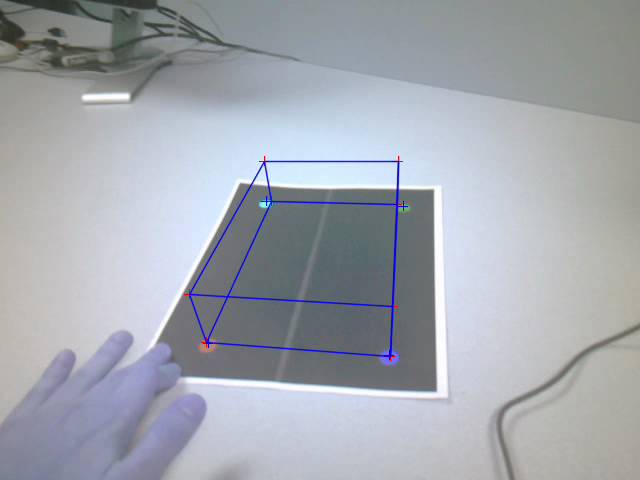
Figure: Inaccurate pose estimation due to marker blurring

In some cases, when the marker detector failed to detect all the feature points, the resulting projection is way off.

There is a slight error in the reprojection of the 4 marker points back into the image from their ideal location in the 3D scene. This can be seen in the screenshots, where the points for the back two features are slightly closer together in the reprojection compared to in the camera. This could be due to a variety of factors: One, we did not correct for radial distortion in the picture, so the visualized points in the image may not actually be on a plane. Second, there is a bit of wiggle room within each marker circle for the point we detect as the feature. As a result, the four feature points may not form a rectangle exactly in the real world, either. Since this error is consistent, it is likely due to a correctable source. Calibration of the camera intrinsics to take into account a first-order approximation of radial distortion may be a good idea in the future. As for the second cause, fixing that would involve coming up with a better feature.

The primary issue, then, was the quality of the feature detector. Using 4 colors as features is highly limiting, as that meant the scene could not contain any other thing in those pixel ranges. This effectively limited the scenes with which we could project objects to white tabletops. Having 4 colors, however, allowed us to quickly identify which feature point corresponded to which point on the real marker. This meant that we did not have to find more than 4 feature points, and most importantly, that we did not have to do something slow like RANSAC to find an agreeable match. Nevertheless, if we limited our features to a small number, we may be able to do a quick RANSAC to find matches without relying on color to differentiate. This would alleviate a lot of problems without current detector, which could reliably pick up colors like red or yellow but had a harder time with green or blue.

Future work on the application can also leverage the strong location dependence of successive camera frames to aid in marker detection. Doing so may provide significant improvements in robustness and performance, as long as the camera does not move around too quickly.

A feature we would have liked to implement would have been an option to manually specify the marker dots in an image. If the user could take an image and mark the four points with the stylus, then our system could have calculated temporary threshold values for that particular lighting scenario, improving the accuracy of the marker detector. A second method to gather such information would be to have user take a picture, have the system mark the marker dots and ask the user if its marks are correct. If not, the process could be repeated. Because our system has demonstrated a competent level of marker detection, it would not take more than 3 or 4 images before the system correctly labeled the dots.

3 videos have been provided as well to show the real time pose estimation using pre-defined markers. Since the frame rate was very small (approximately 1.5-2 frames per second) the video appears to be very fast.

Citations

1) R. Haralick, H. Joo, C. Lee, X. Zhuang, V. Vaidya, M. B. Kim, Pose Estimation from Corresponding Point Data, IEEE Transactions on Systems, Man. And Cybernetics, Vol 19, NO 6

2) R. Horaud, B. Conio, O. Leboulleux, B. Lacolle, An analytic solution for the perspective 4-point problem, IEEE Computer Vision and Pattern Recognition, 1989.

3) C. Lu, G. D. Hager, E. Mjolsness, Fast and Globally Convergent Pose Estimation from Video Images, IEEE Transactions on Pattern Analysis and Machine Intelligence, Vol 22, No 6

4) R. Yu, T. Yang, J. Zheng, X. Zhang, Real-Time Camera Pose Estimation Based on Multiple Planar Markers, 2009 Fifth International Conference on Image and Graphics

5) M. Dhome, M. Richetin, J. T. Lapreste, and G. Rives, Determination of the attitude of 3D objects from a Single Perspective View, IEEE Trans. Pattern Anal. Mach. Intell.

6) M. Maidi, J. Didier, F. Ababsa, M. Mallem, A performance study for camera pose estimation using visual marker based tracking, Machine Vision and Applications (2010)

7) G. Schweighofer, A. Pinz, Robust Pose Estimation from a Planar Target, IEEE Transactions on Pattern Analysis and Machine Intelligence, Vol 28, No 12

8) G. Simon, A. Fitzgibbon, A. Zisserman, Markerless Tracking using Planar Structures in the Scene, Augmented Reality, 2000, Proceedings

9) I. Reisner-Kollmann, A. Reichinger, W. Pergathofer, 3D Camera Pose Estimation Using Line Correspondences and 1D Homographies, Advances in Visual Computing - 6th International Symposium, ISVC 2010

10) F. Dornaika, C. Garcia, Pose Estimation using Point and Line Correspondences, Real-Time Imaging 5, 215–230 (1999)