 This graph can be represented as an SML datastructure as follows:
We have talked previously about systematic ways of visiting the nodes of trees. We have also seen that the various tree-node visiting orders map naturally to important practical problems. Remember, for example, that the evaluation of a logical expression encoded by an abstract syntax tree can be done most naturally if nodes are visited in post-order order. You have discussed this example in section.
Trees are graphs, so we might naturally wonder whether systematic visiting orders can be defined for nodes of general graphs. The answer is yes, and today we are going to discuss two of them: depth-first search (DFS) and breadth-first search (BFS). Other visiting orders (or searches) exist, often in specialized graphs (see, for example, the A* search).
Note: while we talk about "visiting orders," it is also common to talk about "searches" in both graphs and trees. This is because often we are looking for nodes with special properties, and we want to find them by systematically exploring the graph's nodes. In this sense searches and node-visiting orders are intrisically related.
Before we talk about visiting orders, however, we must explore the issue of graph representations.
A common way to represent graphs is to use adjacency lists. Such a list associates with each vertex v a list of all the vertices adjacent to the respective vertex (i.e. the list of all vertices such that there exists an edge starting at vertex v and ending in one of the nodes included in the adjacency list).
Adjacency lists can be used to represent both directed and undirected graphs. Of course, in the case of undirected graphs the list will be redundant, since if a node exists between vertices v1 and v2, then an edge (in fact, the same one) will exist between vertices v2 and v1. It is possible to optimize adjacency lists so that this redundancy is eliminated - for example, one can only represent edges [v1v2] that are characterized by the fact that node v1 < v2 (assuming that we use numbers to identify nodes). The cost of optimizing the representation of undirected graphs is that searches in such optimized adjacency lists become more complicated. This is a tradeoff that is very typical: saving memory often increases running time, while reducing the running time of an algorithm often requires increased memory consumption. Finally, we note that adjacency lists can be used to represent loops (edges that start and end at the same vertex v).
The vertices adjacent to a particular vertex v can be, in general, in any order. It is not uncommon, however, that a certain ordering is imposed; for example, one can list first adjacent nodes that are "closer" in the graph (say, they correspond to edges with lower weights).
For graphs whose nodes are labeled using integers the definition below defines the adjacecy list type:
type vertex = int
type graph = (vertex * vertex list) list
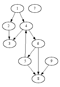
Consider the graph shown below:
This graph can be represented as an SML datastructure as follows:
val g = [(1, [2, 4]), (2, [3]), (3, []),
         (4, [3, 6]), (5, [4, 8]), (6, [5, 8]),
         (7, []), (8, []), (9, [8])]
Let us note that this graph has an isolated node (7), and only one cycle ( 4 -> 6 -> 5 -> 4).
As you know, searching in lists is not very efficient. It is possible to store the adjacency information in datastructures that allow for much faster lookup. Imagine, for example, a binary search tree in which the nodes of the tree store the information identifying the current vertex (say, its number), and the list of its adjacent vertices. The SML type of this "adjacency list" representation could be defined as follows:
type node = vertex * vertex list (* (vertex v) * (adjacency list of v) *)
datatype 'a tree = Empty | Node of 'a tree * 'a * 'a tree
type graph = node tree
Of course, it is clear that only the first component of node (#1 node) should be used for ordering nodes in the tree.
Now, if you imagine that your graph has many nodes, that nodes are added dynamically, and that the numbers identifying newly added nodes are in strictly increasing order, you realize that you need a self-balancing tree, possibly a red-black or a splay tree to store the adjacency information of your graph. And this is how everything comes together...
Other graph representations are possible. A frequent alternative method is that of the adjacency matrix. If the graph has N vertices, its adjacency matrix A has size NxN. The (i,j)th entry of the graph is set to 1 if and only if there exists an edge between vertices vi and vj. Since only one bit is needed to encode the existence of an edge, adjacency graphs can be stored very efficiently. In modern computers (long) integers are represented on 32 bits - an adjacency matrix can store information on 32 edges in this space.
In an undirected graph the adjacency matrix will contain redundant information. If loops are not allowed, this redundancy allows for us to store only the part of the matrix under (or over) the main diagonal. Thus, the number of bits to be represented decreases fron N2 to 1/2*N*(N-1); a significant saving when N is large.
In many important applications one must work with graphs having hundreds of thousands or even millions of nodes which have the property that each vertex is connected to only a few other vertices (say, at most k). Such graphs are common in computer-aided design (CAD) applications, and can be stored very efficiently in a "truncated" adjacency matrix, which keeps only k diagonals above (and below, if the graph is directed) the main diagonal of the adjacency matrix.
Before we define depth-first searches, let us introduce the following terms:
Before we continue, we must first point out the limitations of this terminology. In general graphs a vertex can have more than one parent, i.e. we can arrive at a node following different edges starting at different nodes. Because the parent vertex is not unique, a node's set of siblings will not be unique either. To make things worse, it is possible for a vertex to simultaneously be the sibling and the child of the current node, for example.
We define a depth-first search in a graph as any systematic search in which the children of the current node are examined (or visited) before the siblings of the same node. Note: this definition ignores a few obvious problems, e.g. the fact that the child of the current node might have already been visited.
From the definition above it is clear that in general the depth-first search is not unique.
The definition of the depth-first search captures the intuitive meaning of a search that is "trying" to move far away from the initial node as quickly as possible (note that we measure distance in terms of edges from the current node to the initial node of the search).
A possible implementation of the depth-first search is given below:
fun dfs (g: graph) (n: vertex): vertex list =
  let
    fun helper (todo: vertex list) (visited: vertex list): vertex list =
    case todo of
      [] => []
    | h::t => if (List.exists (fn x => x = h) visited)
                then helper t visited
                else
                  let
                    val adj = case List.find (fn (n, _) => n = h) g of
                                NONE => raise Fail "incomplete adjacency list"
                              | SOME (_, adj) => adj
                  in
                    h :: (helper (adj @ t) (h::visited))
                  end
  in
    helper [n] []
  end
Note: The dfs function shows nodes in the order in which they were visited. The function is recursive, but not tail-recursive. Can you make it into a tail-recursive function?
Before we discuss this algorithm, we once again remind the reader that using lists to store adjacency information and to keep track of the visited nodes is not efficient for graphs with a large number of nodes. We keep this representation because it is very simple, and because at this stage we do not focus primarily on performance issues, but on understanding the search algorithms themselves.
The DFS algorithm shown above maintains a list of vertices to examine (the todo list), as well as a list of vertices that have already been visited (examined, or processed). At each stage, the head h of the todo list is retrieved.
If vertex h has not been visited before, then we retrieve the list of nodes adjacent to it, and we prepend this list to the tail of the todo list. In other words, the todo list is changed so that the current vertex h is removed from it, and the list of all vertices adjacent to h is added to the front of the todo list, minus vertex h. Adding new vertices to the front of the list assures that the children of the current node are processed before its siblings. Before we continue processing the todo list, we expand the list of visited vertices by prepending to it vertex h.
If vertex h has been visited before, then it is simply discarded and the processing of the todo list continues by removing and analyzing the next vertex from the list.
The algorithm shown above does not process the graph's vertices in any particular way; all it does is to retain the order in which nodes were visited. In general, nodes (or edges that lead to these nodes) would be analyzed to extract the information that motivated the search.
We show below the results function dfs produces when a DFS search is initiated from various nodes of the graph shown in the diagram above:
- dfs g 1;
val it = [1,2,3,4,6,5,8] : node list

- dfs g 5;
val it = [5,4,3,6,8] : node list

- dfs g 7;
val it = [7] : node list
It is important to recognize that the visiting order imposed by the DFS search algorithm depends on the node where the search starts, and on the order in which nodes are listed in the adjacency list. Also, a DFS search will stay within the connected component in which it started. Unless you know a priori that your graph it connected, you can not be sure that a DFS search will ultimately reach all nodes. One way to deal with limitation is to start DFS searches from all nodes of a graph. This will guarantee that all nodes are visited, but if the graph has only a small number of connected components, it will lead to the repeated visitation of the same vertices. This wastefulness can be mitigated by further optimizations.
If you examine the DFS algorithm, you might be tempted to "optimize" it by adding to the todo list only the vertex adjacent to the current vertex h that are not already in the visited list. Here is one possible implementation of this idea:
fun dfs (g: graph) (n: vertex): vertex list =
  let
    fun helper (todo: vertex list) (visited: vertex list): vertex list =
    case todo of
      [] => []
    | h::t => let
                val adj = case List.find (fn (n, _) => n = h) g of
                            NONE => raise Fail "incomplete adjacency list"
                          | SOME (_, adj) => adj
                val new = foldr (fn (a, acc) =>
                                  if (List.exists (fn x => x = a) visited)
                                  then acc
                                  else a::acc)
                                []
                                adj
              in
                h :: (helper (new @ t) (h::visited))
              end
  in
    helper [n] []
  end
Note: We used foldr to preserve the order in which nodes are added to the todo list, assuming that they are not already in the visited list.
In the function above only new vertices adjacent to h are added to the todo list. This "optimization," however, changes the order in which nodes are visited. It is simple to see that this is the case. Consider a vertex v that is already in the todo list, but it is also in the list of vertices adjacent to h. Assuming that we are using the correct dfs function (the first one we presented), vertex v would be added for the second time to todo. This assures that all vertices between the two occurences of v in the todo list are processed after vertex v (assuming that they will not be added to the todo list before the first occurence of v). The "optimized" version of the DFS algorithm, however, makes sure that these vertices will be processed before vertex v.
It is possible to optimize the todo list, but that involves the removal of any old occurence of vertex v when a new occurence of the same vertex is prepended to the todo list. The simple approach of discarding an already visited vertex from the todo list is the one typically preferred, however.
Finally, let us examine a third version of the DFS algorithm:
fun dfs (g: graph) (n: vertex): vertex list =
  let
    fun helper (todo: vertex list) (visited: vertex list): vertex list =
    case todo of
      [] => visited
    | h::t => if (List.exists (fn x => x = h) visited)
              then helper t visited
              else
               foldl (fn (v, visited) => helper (v::todo) visited)
                     (h::visited)
                     (case List.find (fn (n, _) => n = h) g of
                        NONE => raise Fail "incomplete adjacency list"
                      | SOME (_, adj) => adj)
  in
    helper [n] []
  end
This version processes the vertices in the adjacency list of vertex h vertex-by-vertex. Note how useful is foldl to implement what is essentially a loop containing recursive calls to function helper. Without running the code, can you predict the relationship between the value of the visited list returned by the first implementation of DFS and the value of the same list returned by this last version? If not, run a few searches through SML, and try to explain the results that you see.
We define a breadth-first search (BFS) in a graph as any systematic search in which the syblings of the current vertex are examined (or visited) before the children of the same node.
The definition of the breadth-first search captures the intuitive meaning of a search that is "trying" to stay as close as possible to the initial node (note that we measure distance in terms of edges from the current node to the initial node of the search).
Breadth-first searches can be analyzed in a manner analogous to that of depth-first searches presented above. We will not repeat the analysis here, rather, we provide one possible SML implementation of BFS:
fun bfs (g: graph) (n: vertex): vertex list =
let
  fun helper (todo: vertex list) (visited: vertex list) =
    case todo of
      [] => []
    | h::t => if (List.exists (fn x => x = h) visited)
              then helper t visited
              else
                let
                  val adj = case List.find (fn (n, _) => n = h) g of
                            NONE => raise Fail "incomplete adjacency list"
                          | SOME (_, adj) => adj
                in
                  h :: (helper (t @ adj) (h::visited))
                end
in
  helper [n] []
end
For the graph whose structure we provided in the diagram above, the bfs search algorithm will return the following results:
- bfs g 1;
val it = [1,2,4,3,6,5,8] : node list

- bfs g 5;
val it = [5,4,8,3,6] : node list

- bfs g 7;
val it = [7] : node list
Now that we are familiar with searches in general graphs we return to the question of the relationship between tree searches and graph searches. Consider the tree represented below:
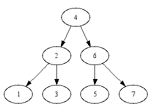
One possible adjacency-list representation of this graph is
val tree = [(1, []), (2, [1, 3]), (3, []),
            (4, [2, 6]),
            (5, []), (6, [5, 7]), (7, [])]
Let us examine the output of the DFS and BFS procedures on this tree, when we start the search at its root (we are using the first version of DFS that was given above):
- dfs tree 4;
val it = [4,2,1,3,6,5,7] : node list

- bfs tree 4;
val it = [4,2,6,1,3,5,7] : node list
This example seems to suggest that the DFS search corresponds to the pre-order visiting order in binary trees, while the BFS search has no equivalent among the tree searches that we have discussed. It is worth pointing out that the BFS search applied to trees results in a systematic, level-by-level examination of the tree, when the search is started from the root: nodes at depth n are examined before nodes at depth n+1.
We must add a caveat to the equivalence between DFS and pre-order searches. The equivalence is predicated upon listing the children of nodes in the tree in the "right" order in the adjacency lists: left child first, followed by the right child.
Indeed, consider the following to alternative representations of the tree at hand:
val tree2 = [(1, []), (2, [3, 1]), (3, []),
             (4, [2, 6]),
             (5, []), (6, [5, 7]), (7, [])]

val tree3 = [(1, []), (2, [3, 1]), (3, []),
             (4, [6, 2]),
             (5, []), (6, [7, 5]), (7, [])]
The DFS algorithm will now produce the following output:
- dfs tree2 4;
val it = [4,2,3,1,6,5,7] : node list

- dfs tree3 4;
val it = [4,6,7,5,2,3,1] : node list
For tree3, the DFS algorithm produces a visiting order that corresponds to the pre-order search in a tree that is the "mirror image" of tree. For tree2 there is no correspondence between pre-order visits and DFS, unless we would want to extend the concept of "mirroring" to subtrees.