Lecture 20: Recursion Trees and the Master Method

Recursion Trees

A recursion tree is useful for visualizing what happens when a recurrence is iterated. It diagrams the tree of recursive calls and the amount of work done at each call.

For instance, consider the recurrence

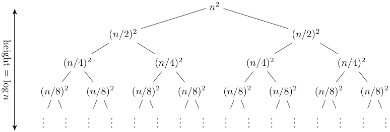
T(n) = 2T(n/2) + n².

The recursion tree for this recurrence has the following form:

In this case, it is straightforward to sum across each row of the tree to obtain the total work done at a given level:

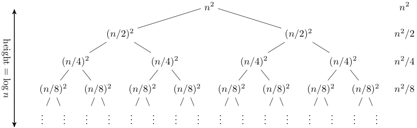
This a geometric series, thus in the limit the sum is O(n²). The depth of the tree in this case does not really matter; the amount of work at each level is decreasing so quickly that the total is only a constant factor more than the root.

Recursion trees can be useful for gaining intuition about the closed form of a recurrence, but they are not a proof (and in fact it is easy to get the wrong answer with a recursion tree, as is the case with any method that includes ''...'' kinds of reasoning). As we saw last time, a good way of establishing a closed form for a recurrence is to make an educated guess and then prove by induction that your guess is indeed a solution. Recurrence trees can be a good method of guessing.

Let's consider another example,

T(n) = T(n/3) + T(2n/3) + n.

Expanding out the first few levels, the recurrence tree is:

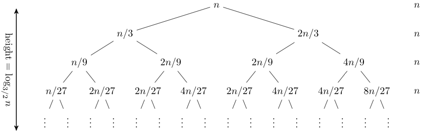
Note that the tree here is not balanced: the longest path is the rightmost one, and its length is log_3/2 n. Hence our guess for the closed form of this recurrence is O(n log n).

The Master Method

The master method is a cookbook method for solving recurrences. Although it cannot solve all recurrences, it is nevertheless very handy for dealing with many recurrences seen in practice. Suppose you have a recurrence of the form

T(n) = aT(n/b) + f(n),

where a and b are arbitrary constants and f is some function of n. This recurrence would arise in the analysis of a recursive algorithm that for large inputs of size n breaks the input up into a subproblems each of size n/b, recursively solves the subproblems, then recombines the results. The work to split the problem into subproblems and recombine the results is f(n).

We can visualize this as a recurrence tree, where the nodes in the tree have a branching factor of a. The top node has work f(n) associated with it, the next level has work f(n/b) associated with each of a nodes, the next level has work f(n/b²) associated with each of a² nodes, and so on. At the leaves are the base case corresponding to some 1 ≤ n < b. The tree has log_bn levels, so the total number of leaves is a^log_bn = n^log_ba.

The total time taken is just the sum of the time taken at each level. The time taken at the i-th level is aⁱf(n/bⁱ), and the total time is the sum of this quantity as i ranges from 0 to log_bn−1, plus the time taken at the leaves, which is constant for each leaf times the number of leaves, or O(n^log_ba). Thus

T(n) = Σ_0≤i<logbn aⁱf(n/bⁱ) + O(n^log_ba).

What this sum looks like depends on how the asymptotic growth of f(n) compares to the asymptotic growth of the number of leaves. There are three cases:

• Case 1: f(n) is O(n^{log_ba − ε}). Since the leaves grow faster than f, asymptotically all of the work is done at the leaves, so T(n) is Θ(n^{log_b a}).
• Case 2: f(n) is Θ(n^log_ba). The leaves grow at the same rate as f, so the same order of work is done at every level of the tree. The tree has O(log n) levels, times the work done on one level, yielding T(n) is Θ(n^{log_b a} log n).
• Case 3: f(n) is Ω(n^{log_ba + ε}). In this case f grows faster than the number of leaves, which means that asymptotically the total amount of work is dominated by the work done at the root node. For the upper bound, we also need an extra smoothness condition on f in this case, namely that af(n/b) ≤ cf(n) for some constant c < 1 and large n. In this case T(n) is Θ(f(n)).

As mentioned, the master method does not always apply. For example, the second example considered above, where the subproblem sizes are unequal, is not covered by the master method.

Let's look at a few examples where the master method does apply.

Example 1 Consider the recurrence

T(n) = 4T(n/2) + n.

For this recurrence, there are a=4 subproblems, each dividing the input by b=2, and the work done on each call is f(n)=n. Thus n^log_ba is n², and f(n) is O(n^2-ε) for ε=1, and Case 1 applies. Thus T(n) is Θ(n²).

Example 2 Consider the recurrence

T(n) = 4T(n/2) + n².

For this recurrence, there are again a=4 subproblems, each dividing the input by b=2, but now the work done on each call is f(n)=n². Again n^log_ba is n², and f(n) is thus Θ(n²), so Case 2 applies. Thus T(n) is Θ(n² log n). Note that increasing the work on each recursive call from linear to quadratic has increased the overall asymptotic running time only by a logarithmic factor.

Example 3 Consider the recurrence

T(n) = 4T(n/2) + n³.

For this recurrence, there are again a=4 subproblems, each dividing the input by b=2, but now the work done on each call is f(n)=n³. Again n^log_ba is n², and f(n) is thus Ω(n^2+ε) for ε=1. Moreover, 4(n/2)³ ≤ kn³ for k=1/2, so Case 3 applies. Thus T(n) is Θ(n³).

Example: Yet Another Sorting Algorithm

The following function sorts the first two-thirds of a list, then the second two-thirds, then the first two-thirds again:

let rec sort3 (a : 'a list) : 'a list =
  match a with
      [] -> []
    | [x] -> [x]
    | [x; y] -> [(min x y); (max x y)]
    | _ -> 
	let n = List.length a in
	let m = (2*n + 2)/3 in
	let res1 = sort3 (take a m) @ (drop a m) in
	let res2 = (take res1 (n-m)) @ sort3 (drop res1 (n-m)) in
	  sort3 (take res2 m) @ (drop res2 m)

Here take a m is the list consisting of the first m elements of a, and drop a m is the list consisting of all but the first m elements of a. Perhaps surprisingly, this algorithm does sort the list. We leave the proof that it sorts correctly as an exercise. The key is to observe that the first two passes ensure that the last third of the list contains the correct elements in the correct order.

We can derive the running time of the algorithm from its recurrence using the master method. The routine does O(n) work in addition to three recursive calls on lists of length 2n/3. Therefore its recurrence is:

T(n) = cn + 3T(2n/3)

If we apply the master method to the sort3 algorithm, we see that we are in case 1, so the algorithm is O(n^log_3/23) = O(n^2.71), making it even slower than insertion sort! Note that being in Case 1 means that improving f(n) will not improve the overall time. For instance, replacing lists with arrays improves f(n) to constant from linear time, but the overall asymptotic complexity is still O(n^2.71).